Overview
This page provides a short tutorial for the online analysis interface for INTEGRAL/JEM-X data.
More details can be found on the AstrODA paper. This is a web interface runs the OSA INTEGRAL analysis on servers of the University of Geneva.
Details on INTEGRAL analysis can be found at the ISDC pages.
It is possible to use this platforn without registering, but unregistered users, the limit is of 50 science windows. Registered users can process up to 500 science windows. It is also possible to increase this limit for scientific projects with UNIGE participation.
Registered users will receive an email at job submission and one at its completion with a permanet URL to the product and python code to make the same request.
A query for which results are available will finish in a few seconds, others will require a variable time, from minutes to hours for large requests.
Source query panel
Top panel of the interface defines parameters of analysis not specific to JEM-X. You can select a source and a time interval. The tool will select for you
at most 50 science windows within your time interval.
Instrument query panel
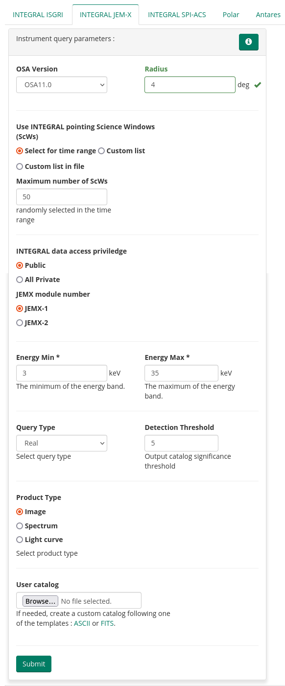
JEM-X specific parameters appear when "INTEGRAL JEM-X" button is selected in the virtual desktop field. A box with parameters for imaging, spectral and timing analysis appears in this case.
Note the specificity to select one JEM-X unit.
As for ISGRI, it is possible to select randomly a number of science windows from a time interval, to specify a list of science windows, or to upload a file with the list of science windows.
One can access public or public+private data, the latter only if logged in with custom privileges after agreeing on the line of conduct.
The maximum and minimum energies are relative to imaging and light curves, while spectra are extracted on 16 pre-defined energy bins
Analysis thread
A generic analysis flow typically starts from Imaging analysis and proceeds through Imaging -> Speactral/Timing analysis chains. Spectral and timing analysis steps rely on results of the imaging analysis (on catalog of sources found in imaging analysis) and it is recommended to always start from the imaging analysis step and refine the catalog. Note that for part of the mission, only one of the two JEM-X modules was active in alternance. One can check from the INTEGRAL Archive Query page which one was active at a give time, or one can try with one unit and then the other one. The analysis steps are described below:
QUERY DATA
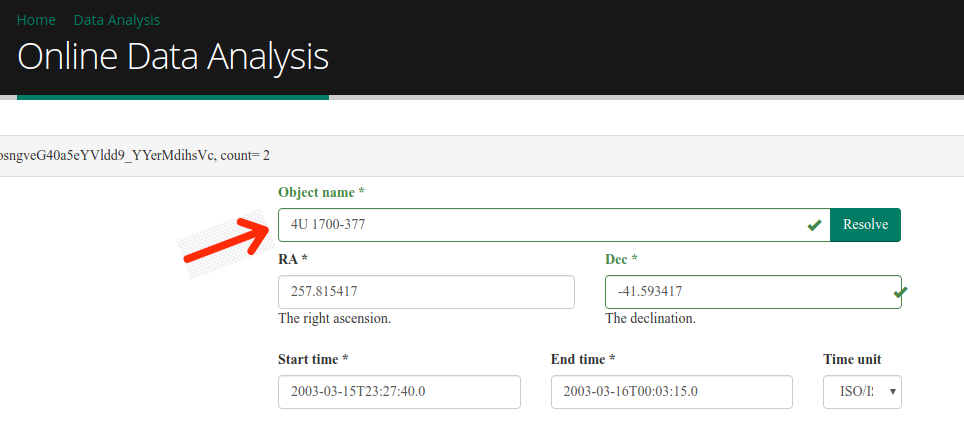
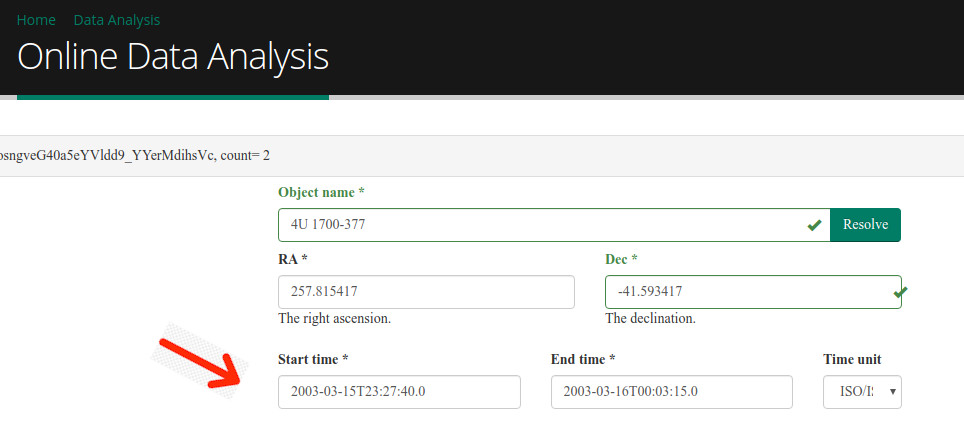
- Start analysis from choosing the source name of interest and resolve the coordinates with the "Resolve" button.
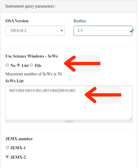
- Define time interval for the data. This could be done either in the "Start time" / "End time" fields in the multi-instrument top panel or by providing the list of telescope pointings (Science Windows, SCW) in the dedicated parameter box in parameter box in INTEGRAL JEM-X panel (Format is "219900320010.001,219900330010.001"). Note that SCW list input overrides the generic time interval input. Maximum number of SCWs is currently limited to 50 in the list.
IMAGING ANALYSIS
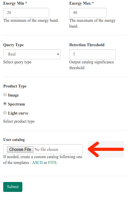
- Select "Image" checkbox and enter the energy interval for image extraction. Note that the analysis results are cached and entering "standard" energy bounds (e.g. 3-20 keV) might speed up the analysis because exsiting results would be evoked from cache memory rather than produced from scratch).
- The "detection threshold" is used for the compilation of the catalog.
- Launch imaging analysis by pressing "Submit" button at the bottom of the INTEGRAL JEM-X parameter panel.
- Unregistered users can wait or resubmit the same query, registered users will receive an email upon submittion and one upon completion.
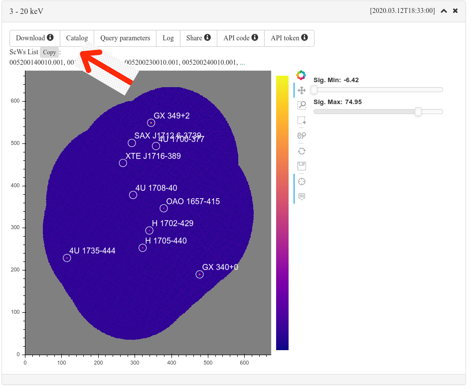
- Mosaic image is displayed in the centre of workspace. Inspect the image to check if your source of interest is detected.
- Optionally enter parameters for image and imaging results display: limits for the minimum and maximum significance which define the image color scale and minimal significance of detected source to be displayed.

- Click on "catalog" button. If your source of interest is detected in mosaic with significance higher than previously defined significance threshold, the source should appear in the catalog. You also have an option to download the catalog in FITS or ASCII format for further analysis.
SPECTRAL ANALYSIS
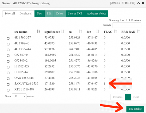
- Prepare the catalog for the spectral analysis from an image result. When you check a source, you can make an operation on it, like deleting. You can edit values.
- We suggest to set "FLAG" to 1 for the source of interest to force the spectral or light curve extraction in a single science window.
- Uncheck all sources and click on "use catalog".
- The catalog which appears will be used for the analysis when you click on "use catalog". Note that you can also load a catalog, extracted for instance with ISGRI.

If "Use catalog" is not clicked. the full imaging catalog will be given as input for the spectral analysis, but without "FLAG" selection. Spectra of all sources found in imaging will be generated (processing might take more time in this case). If there sources brighter than your source of interest in the mosaic image it is advised to include at least all the brighter sources in the spectral analysis. Otherwise the spectrum of the source of interest could not be reliable. - Check the "Spectum" box in INTEGRAL JEM-X parameter field.
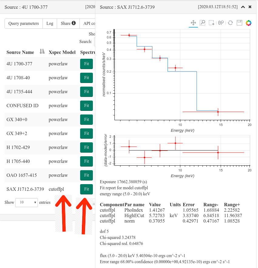
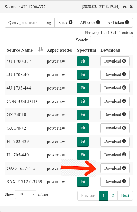
- Launch spectral analysis by clicking "Submit" button. Once the analysis is done, a panel with the list of sources for which the spectra were produced displays in the centre of the INTEGRAL JEM-X workspace. You could click on "fit" button next to your source of interest to see the results of the analysis. At this stage you can choose the spectral model. Results includes a plot of the spectrum and the result of the spectral model fitting in XSPEC.

- You also have a possibility to download the spectrum in FITS format for further analysis.


TIMING ANALYSIS
-
Check the "Lightcurve" checkbox. An additional set of parameters for lightcurve production shows up at the bottom of INTEGRAL JEM-X parameter panel. Enter the width of the time bin for the lightcurve. The Start and end time of the lightcurve are determined by the time limits set in the top multi-instrument panel or by the list of SCWs in the INTEGRAL JEM-X parameter panel. There is no maximal length of the time bin in the lightcurve, but it is highly suggested not to exceed one science windew typical duration (~2 ks). The minimum bin is 4 s.
-
The selection of sources for the timing analysis is performed identically to the spectral analysis, above.
-
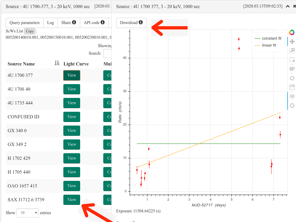
Launch the lightcurve extraction by pressing "Submit" button. Once the lightcurve is produced, the list of sources is displayed in the center of the workspace. One has to click on "view" to see the light curve together with the result of fitting on constant and linear function. You have a possibility to download the lightcrve in FITS OGIP-compliant format for further analysis.