Studying equilibria in a resonant chain#
In this notebook we search for families of equilibrium configurations (fixed points of the averaged problem) of a resonant chain. We search for the position of these equilibria as a function of the parameter delta (see Delisle 2017). To try and find all possible families, we first launch many times a root-finding algorithm with random starting points in the parameter space, for a rough grid on delta. Once this is done, we perform a second search with with a finer grid on delta, trying to follow the discovered families. We then compute the eigen-values and eigen-modes around each fixed point. This allows to check if the equilibria are stable (elliptical fixed points, with purely imaginary eigen-values) or unstable (hyperbolic fixed points).
[1]:
from multiprocessing import Pool

import matplotlib.pyplot as plt
import numpy as np
from celeries import mmr
[2]:
# Initialize the MMR model
m0 = 1.0  # Stellar mass (in Solar mass)
mp = np.array([1e-5, 1e-5, 1e-5])  # planets masses (in Solar mass)
k = np.array(
  [[2, 3], [3, 4]]
)  # Resonance coefficients (here a 3/2 MMR for the inner couple and a 4/3 for the outer couple)
deg = 1  # degree of the development of the Hamiltonian in eccentricities

Hmmr = mmr.MMR(m0, mp, k, deg)
[3]:
# First search of fp families
delta_rough = np.linspace(0, 1e-4, 5)  # rough grid in delta
ntry = 2_500  # number of root-finding search per delta value

# Generate random starting points
np.random.seed(0)
rand_v0 = np.array([Hmmr.random_v0(dk, ntry) for dk in delta_rough])

# Parallel search (using multiprocessing)
nproc = 16


# We launch ntry search for each value of delta
def search_job(kjob):
  kd, kt = kjob // ntry, kjob % ntry
  return Hmmr.solve_fp(rand_v0[kd, kt], delta_rough[kd])


with Pool(nproc) as pool:
  sols_rough = np.array(pool.map(search_job, np.arange(rand_v0[..., 0].size))).reshape(
    (-1, ntry)
  )

# Merge all these results to identify fp families
v_fp_rough = Hmmr.merge_fp(sols_rough)
[4]:
# Second search to follow the families on a finer grid
delta = np.linspace(-5e-5, 1e-4, 401)

krough = np.argwhere(np.isfinite(v_fp_rough[:, :, 0]))


# Continuation of each family (in parallel)
def follow_job(kfp):
  # Try to follow a fp family
  # Follow the family with decreasing delta
  v0 = v_fp_rough[*krough[kfp]]
  kd0 = np.argmin(np.abs(delta - delta_rough[krough[kfp, 0]]))
  sols = []
  for kd in range(kd0, -1, -1):
    sol = Hmmr.solve_fp(v0, delta[kd])
    sols.insert(0, sol)
    if sol.success:
      v0 = sol.x
  # Follow the family with increasing delta
  v0 = v_fp_rough[*krough[kfp]]
  for kd in range(kd0 + 1, delta.size):
    sol = Hmmr.solve_fp(v0, delta[kd])
    sols.append(sol)
    if sol.success:
      v0 = sol.x
  return sols


with Pool(nproc) as pool:
  sols = np.array(pool.map(follow_job, np.arange(krough.shape[0]))).T

# Merge these results to identify fp families
v_fp = Hmmr.merge_fp(sols)
print(f'Found {v_fp.shape[1]} families')
Found 12 families
[5]:
# Convert fp coordinates to usual elliptical elements (a, e, \lambda, \varpi)
ell = np.array([[Hmmr.v2ell(vkl, dk, 1) for vkl in vk] for dk, vk in zip(delta, v_fp)])
[6]:
# Compute eigenvalues/modes around the fp
eigen = [
  [
    Hmmr.fp_modes(vkl, dk)
    if np.isfinite(vkl[0])
    else (np.full(vkl.size, np.nan), np.full((vkl.size, vkl.size), np.nan))
    for vkl in vk
  ]
  for dk, vk in zip(delta, v_fp)
]

eig_val = np.array([[ekl[0] for ekl in ek] for ek in eigen])
eig_vec = np.array([[ekl[1] for ekl in ek] for ek in eigen])

# Check if fp is elliptic (stable) or hyperbolic (unstable)
stab = np.all(np.abs(eig_val.real) / (1e-40 + np.abs(eig_val.imag)) < 1e-5, axis=-1)
v_stab = v_fp.copy()
v_stab[*(np.argwhere(~stab).T)] = np.nan
ell_stab = ell.copy()
ell_stab[*(np.argwhere(~stab).T)] = np.nan
eig_val_stab = eig_val.copy()
eig_val_stab[*(np.argwhere(~stab).T)] = np.nan

v_unstab = v_fp.copy()
v_unstab[*(np.argwhere(stab).T)] = np.nan
ell_unstab = ell.copy()
ell_unstab[*(np.argwhere(stab).T)] = np.nan
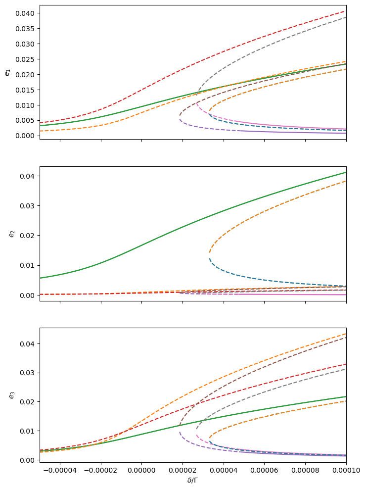
[7]:
# Plot equilibrium eccentricities (unstable equilibria in dashed lines)
_, axs = plt.subplots(Hmmr.npla, 1, sharex=True, figsize=(8, 4 * Hmmr.npla))
for p in range(Hmmr.npla):
  ax = axs[p]
  for els, ls in [(ell_stab, '-'), (ell_unstab, '--')]:
    ax.set_prop_cycle(None)
    ax.plot(delta, els[:, :, p, 1], ls)
  ax.set_ylabel(f'$e_{p + 1}$')
ax.set_xlim(delta[0], delta[-1])
ax.set_xlabel('$\\delta / \\Gamma$')
plt.show()
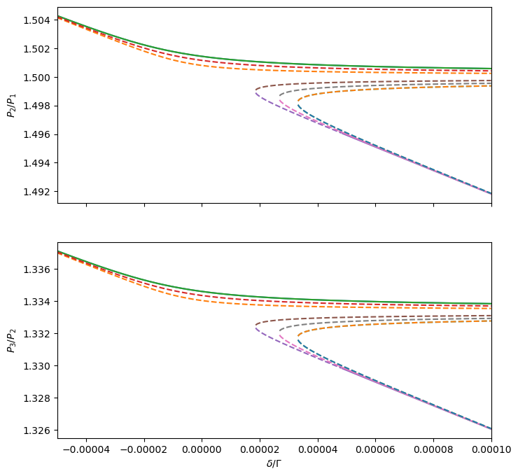
[8]:
# Plot period ratios
_, axs = plt.subplots(Hmmr.npla - 1, 1, sharex=True, figsize=(8, 4 * (Hmmr.npla - 1)))
for p in range(Hmmr.npla - 1):
  ax = axs[p]
  for els, ls in [(ell_stab, '-'), (ell_unstab, '--')]:
    ax.set_prop_cycle(None)
    ax.plot(
      delta,
      np.sqrt(
        Hmmr.mu[p] / Hmmr.mu[p + 1] * (els[:, :, p + 1, 0] / els[:, :, p, 0]) ** 3
      ),
      ls,
    )
  ax.set_ylabel(f'$P_{p + 2}/P_{p + 1}$')
ax.set_xlim(delta[0], delta[-1])
ax.set_xlabel('$\\delta / \\Gamma$')
plt.show()
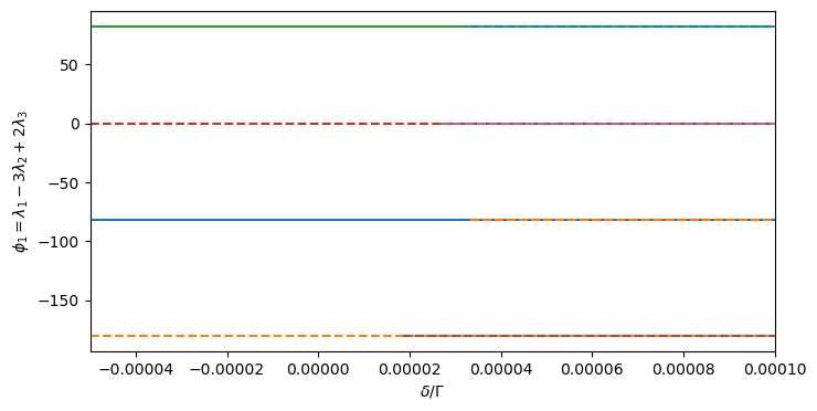
[9]:
# Plot 3-planet resonance angles (Laplace angles)
_, axs = plt.subplots(Hmmr.npla - 2, 1, sharex=True, figsize=(8, 4 * (Hmmr.npla - 2)))
for p in range(Hmmr.npla - 2):
  ax = axs if Hmmr.npla == 3 else axs[p]
  for vs, ls in [(v_stab, '-'), (v_unstab, '--')]:
    ax.set_prop_cycle(None)
    ax.plot(
      delta,
      180
      / np.pi
      * np.array([mmr.continuous_angle(phi) for phi in vs[:, :, Hmmr.npla + p].T]).T,
      ls,
    )
  ax.set_ylabel(f'$\\phi_{p + 1} = {Hmmr.laplace_latex_label(p)}$')
ax.set_xlabel('$\\delta / \\Gamma$')
ax.set_xlim(delta[0], delta[-1])
plt.show()
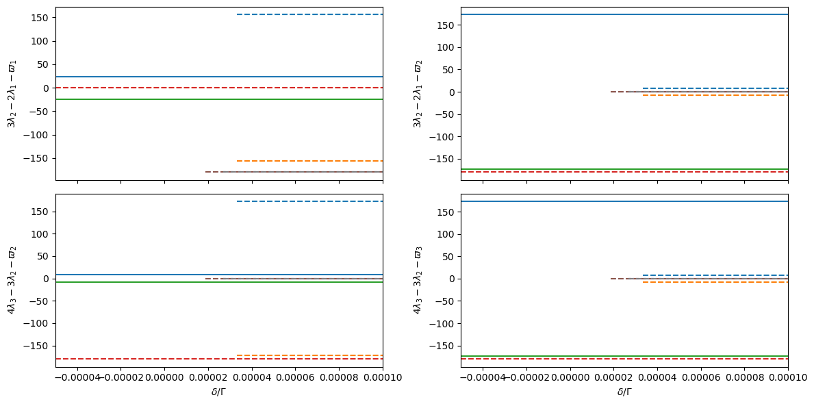
[10]:
# Plot 2-planet resonance angles
_, axs = plt.subplots(Hmmr.npla - 1, 2, sharex=True, figsize=(12, 2 * Hmmr.npla))
for p in range(Hmmr.npla - 1):
  for vs, ls in [(v_stab, '-'), (v_unstab, '--')]:
    sigs = Hmmr.v2couple(vs, p, p + 1)
    for ax, sig in zip(axs[p], sigs):
      ax.set_prop_cycle(None)
      ax.plot(
        delta,
        180 / np.pi * np.array([mmr.continuous_angle(sigk) for sigk in sig.T]).T,
        ls,
      )
  for ax, lbl in zip(axs[p], Hmmr.couple_latex_labels(p, p + 1)):
    ax.set_ylabel(f'${lbl}$')
for ax in axs[-1]:
  ax.set_xlabel('$\\delta / \\Gamma$')
  ax.set_xlim(delta[0], delta[-1])
plt.tight_layout()
plt.show()
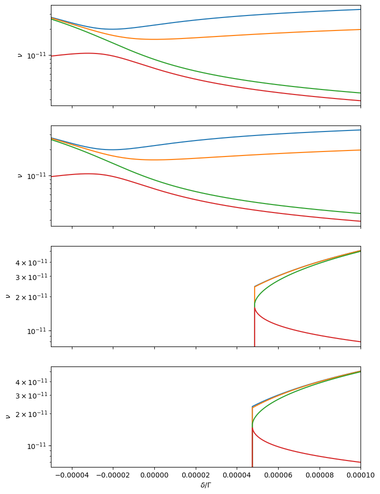
[11]:
# Plot the frequencies of the eigenmodes around the stable equilibria
kfp_stab = np.where(np.any(stab, axis=0))[0]
_, axs = plt.subplots(kfp_stab.size, 1, sharex=True, figsize=(8, 3 * kfp_stab.size))
axs = [axs] if kfp_stab.size == 1 else axs
for ax, kfp in zip(axs, kfp_stab):
  ax.plot(delta, np.abs(eig_val_stab[:, kfp, : Hmmr.ndof].imag))
  ax.set_ylabel('$\\nu$')
  ax.set_yscale('log')
ax.set_xlabel('$\\delta / \\Gamma$')
ax.set_xlim(delta[0], delta[-1])
plt.show()