
2D spectral reduction#
The present tutorial relates to the formatting and cleaning of time-series of 2D echelle spectra, as provided by the DRS of standard spectrographs.
Even if you are only interested in using ANTARESS to analyze a specific spectral range, we recommend processing the full spectra as some corrections benefit from exploiting the maximum information. Spectra can be trimmed) to your range of interest at the end of the spectral reduction.
Once reduced, the spectral time-series can be further processed by the workflow for a variety of purposes, in particular the extraction and analysis of spectra from the stellar and planetary atmospheres.
We illustrate the tutorial with ESPRESSO observations of TOI-421b (on 2022-11-17) and TOI-421c (on 2023-11-06).
We assume that you have already set up your system and dataset.
Calibration and noise estimates#
The first step is the Instrumental calibration module, which defines instrumental calibration profiles used to scale back spectra from flux to extracted count units, and to calculate spectral weight profiles.
The present module is always active in spectral mode. Set it to calculation mode (gen_dic[‘calc_gcal’] = True).
The calibration profiles used by ANTARESS can be defined in two different ways:
If blazed data are available (S2D_BLAZE_A.fits files from ESPRESSO-like DRS) you can store them in the same directory as the input data. Then by activating gen_dic[‘gcal_blaze’]=True the module will use the blazed and input data to retrieve the exact calibration profiles, as well as the detector noise.
If blazed data are not available or if you set gen_dic[‘gcal_blaze’]=False, calibration profiles will be estimated approximately using the input flux and error tables, if available. Detector noise cannot be retrieved.
Blaze-derived calibration profiles may be undefined in some pixels, while estimated profiles typically display high-frequency noise. In such cases, we fit the retrieved profiles with an analytical model. Since calibration profiles have low-frequency variations we first bin them with a spectral bin size gen_dic[‘gcal_binw’] (in \(\\A\)), which should be large enough to capture variations at the edges of the spectral orders and small enough to smooth out noise. Estimated profiles may have low S/R in individual exposures, and can further be fitted over groups of gen_dic[‘gcal_binN’] exposures. The binned calibration profiles are then fitted with the model key gen_dic[‘gcal_mod’] set to:
spline : a 1D smoothing spline, which is the default and preferred option for blaze-derived profiles. You can adjust the smoothing factor with:
gen_dic['gcal_smooth']={'ESPRESSO':1e-3}
custom : a piecewise model consisting of a low-order central polynomial joined with higher-order polynomials on each side to better capture sharp blaze variations at the edges of spectral orders. This model is more robust than a spline to fit estimated profiles. You can control the range covered by the edge polynomials (in fraction of the order range) with:
gen_dic['gcal_edges']={'blue':0.3,'red':0.3}
And the degree of the three polynomials with:
gen_dic['gcal_deg']={'blue':4,'mid':2,'red':4}
Outliers to the binned calibration profiles can be automatically excluded from the fit by setting thresholds applied within orders (‘outliers’) and over all orders (‘global’), for a given instrument.
The best-fit model will be used to extrapolate blaze-derived profiles over undefined pixels, and to fully replace estimated profiles.
You can plot the spectral calibration profiles from each order of the spectrograph (Fig. 11) with plot_dic[‘gcal_ord’]=’pdf’. If blaze profiles are not available Fig. 11 is useful to check that your settings for the module allow estimating correctly the calibration profiles from the input data.
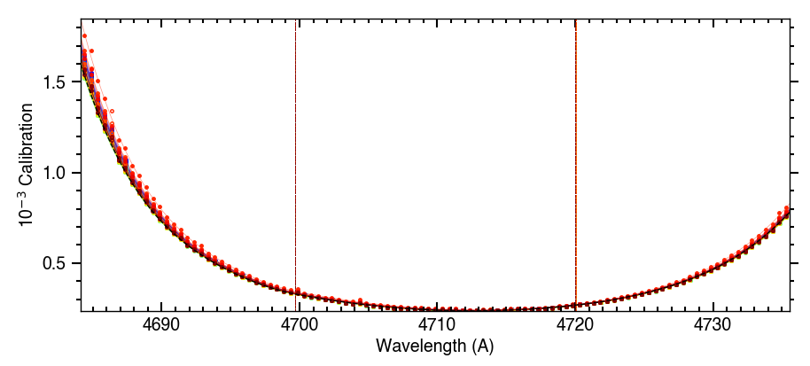
Fig. 11 Calibration profile for a spectral order during the 2023-11-06 visit. Dots and solid lines show the measured and fitted calibration profiles, respectively, for each exposure (colored over the rainbow scale). Vertical lines indicate the transitions between the model piecewise polynomials.#
You can compare the relative noise contributions from photons and from the detector in each order (Fig. 12) with plot_dic[‘noises_ord’]=’pdf’. This provides useful insights into the weights of these two noise sources in various spectral ranges and detector locations.
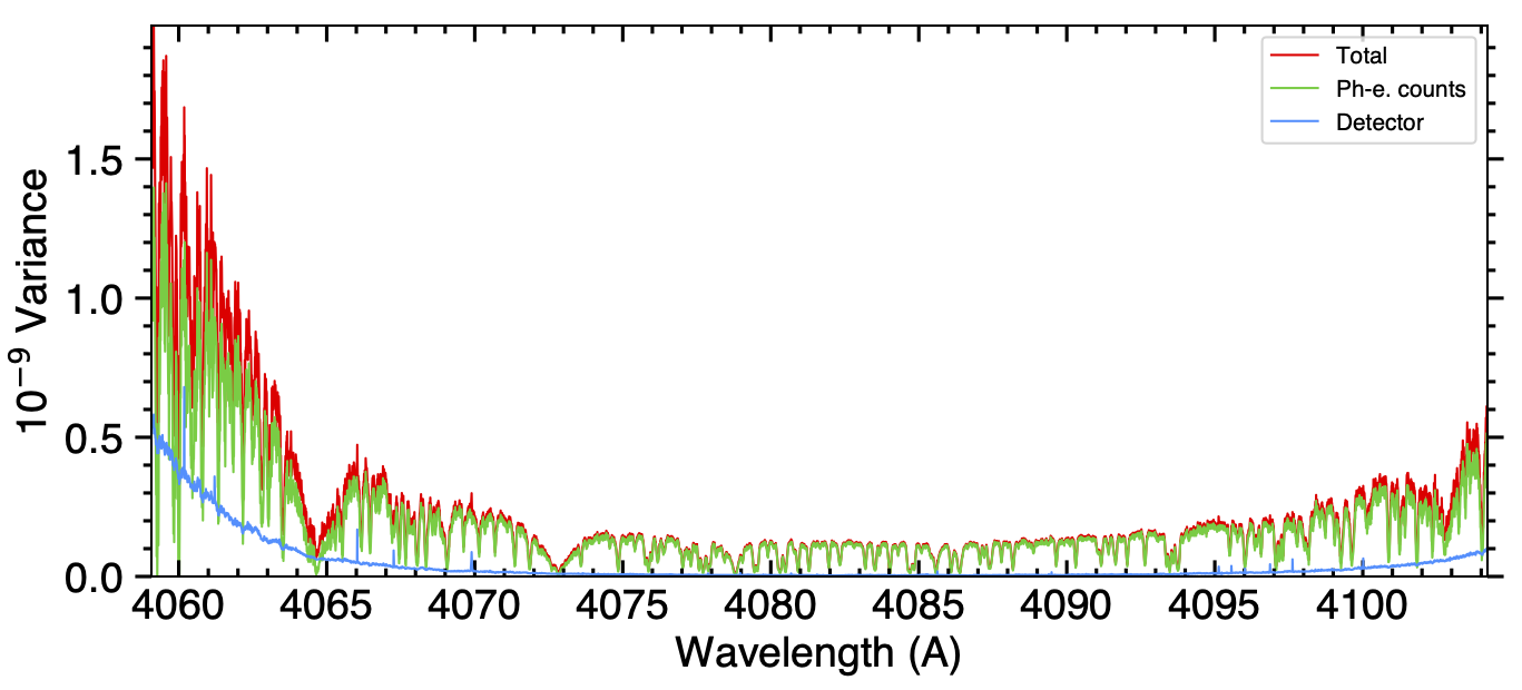
Fig. 12 Variances, in flux units, associated to the spectral density of unblazed counts measured in a blue ESPRESSO order during one of the 2023-11-06 exposures. In regions with lower raw photoelectron counts (at short wavelengths, at the edges of orders, and at the bottom of deep stellar lines) the relative contribution of the detector noise (blue profile) to the total variance (red profile) increases compared to photon noise from the star (green profile).#
Those plots are saved in /Working_dir/Star/Planet_Plots/General/gcal/Instrument/Visit/.
Once you are satisfied with the results of the module, you can set it to retrieval mode (gen_dic[‘calc_gcal’] = False).
Telluric correction#
The next step deals with the correction of telluric absorption lines. The DRS of some spectrographs provide telluric-corrected 2D echelle spectra, in which case you can skip this step - although you may still be interested in comparing both corrections.
The present version of ANTARESS calculates a telluric spectrum from a simple model of Earth atmoshere, computes its CCF over a selection of optimal telluric lines, and fits it to the equivalent CCF from the spectrum measured in each exposure.
This approach exploits two types of static files: a list of telluric lines (mandatory) and a resolution map of the spectrograph (optional).
These files already have default versions for ANTARESS-compatible instruments, and we provide tutorials to optimize the telluric fit linelists and to define resolution maps for additional spectrographs.
In previous versions of the workflow the telluric CCF was computed using uniform weights (gen_dic[‘tell_fit_weights’] = magenta:’unity’). We found that using weigths proportional to the telluric line contrast (gen_dic[‘tell_fit_weights’] = magenta:’intens’) substantially improves the correction, and it is now the default option.
Activate the Telluric correction module (gen_dic[‘corr_tell’] = True) and set it to calculation mode (gen_dic[‘calc_corr_tell’] = True).
Then define which telluric species should be corrected for. Here, we include water and oxygen as:
gen_dic['abstell_species']={'ESPRESSO':['H2O','O2']}
You can check for the convergence of the telluric model fitted to the data by plotting its properties (with plot_dic[‘tell_prop’]=’pdf’), and you can evaluate the fit quality by plotting the telluric CCFs of the model spectrum, observed spectrum, and their difference (with plot_dic[‘tell_CCF’]=’pdf’, see Fig. 14). These plots are saved in /Working_dir/Star/Planet_Plots/Spec_raw/Tell_corr/Instrument_Visit/.
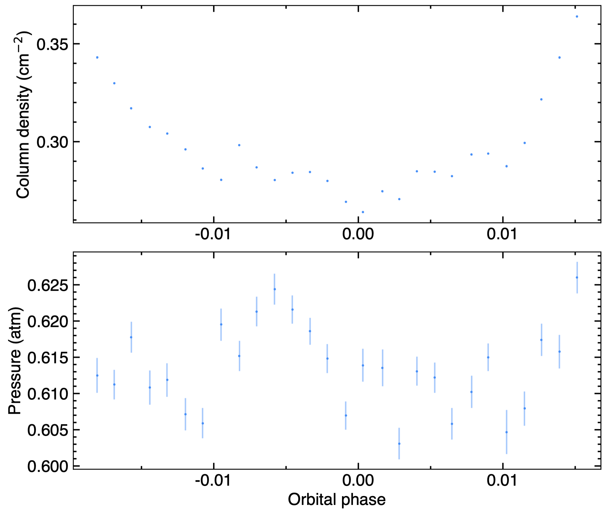
Fig. 13 Telluric water properties derived for the 2023-11-06 visit. The top and bottom panel show the integrated vapour and average pressure along the LOS, respectively, as a function of orbital phase.#
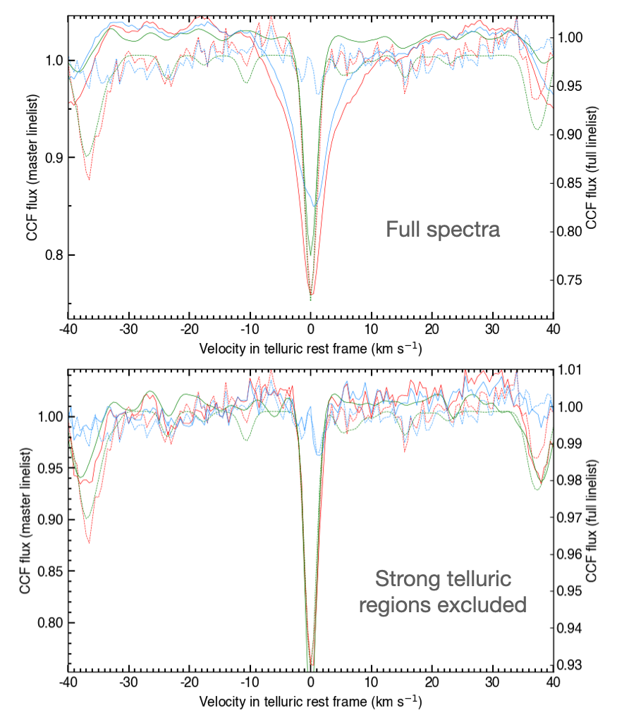
Fig. 14 Top panel: telluric CCF for O2 computed using the entire spectral range. Observed spectrum is shown as red, and blue represent the residuals after correction. Best-fit telluric spectrum is shown in green. Bottom panel: same as top panel but the best fit telluric CCF is computed while excluding regions with strong telluric features.#
An initial run can be made to inspect the telluric correction performed with the default settings. Based on this first run you can then try to activate and adjust several options.
The fitted telluric properties can be finely controlled using:
gen_dic['tell_mod_prop']={instrument:{visit:{molecule:{par: { 'vary' : bool , 'value': float , 'min': float, 'max': float } } } }}
The model properties (par) are described in the configuration file, and the way to control them is described in the fit tutorial.
You can further control the fit range, for example to exclude spurious features from lines close to the CCF mask lines (with rv in the Earth rest frame, in km/s):
gen_dic['tell_fit_range'] = {instrument:{visit:{molecule : [rv0,rv1]}}
Note
While they provide a more realistic fit to the data, the next options may increase computing time while not necessarily improving significantly the correction. You should thus compare outputs from the telluric module and from your later analysis (RV series, transmission spectra, …) to decide whether you need to apply them.
Option 1. The model CCF is computed by default over the telluric spectrum of the fitted species alone. This is not directly comparable with the measured spectrum, which contains stellar lines and possibly telluric lines from other species. You can include stellar lines in the model by providing the path to an ANTARESS-built master spectrum using the gen_dic[‘tell_Fstar_ref’] field (see how to set it up in the configuration file). You can include telluric lines from all fitted species in the model by setting gen_dic[‘tell_fit_mod’] to ‘multi’ instead of the default ‘single’.
Option 2. The telluric lines used to computed the model CCF may saturate in some exposures with high airmass, biasing the fit. By setting gen_dic[‘tell_fit_sat’] = True, a preliminary fit will be performed to flag saturated lines in a given exposure and remove them from the final fit.
Option 3. The continuum of the measured CCF may not be flat like the model one, for example due to broadband spectral variations. You can model the continuum of the model CCF with a polynomial instead of a flat line (with deg between 1 and 4):
gen_dic['tell_CCFcont_deg'] = {instrument:{visit:{molecule : deg}}
And specify the range over which the continuum is defined (with rv in the Earth rest frame, in km/s):
gen_dic['tell_cont_range'] = {instrument:{visit:{molecule : [rv0,rv1]}}
Once the fit is performed you can control how to correct the spectra using your best-fit telluric model. Deep telluric lines are typically not well modelled, resulting in an overcorrection of the spectrum that manifests as an emission spike with potentially broad wings. To compensate for this, you can set to undefined the flux in pixels where the model telluric lines are deeper than a contrast threshold (0 for no absorption, 1 for full absorption):
gen_dic['tell_depth_thresh'] = 0.9
As well as the flux in pixels within ± gen_dic[‘tell_width_thresh’] (in km/s) from the center of telluric lines with core contrast larger than the above threshold.
You can choose which exposures (index idx_exp counted from 0), spectral orders (index idx_ord counted from 0), and spectral ranges (independent wavelength intervals bounded by l in \(\\A\) in the Earth rest frame)) should be corrected for with:
gen_dic['tell_exp_corr'] = {instrument:{visit: [idx_exp] }}
gen_dic['tell_ord_corr'] = {instrument:{visit: [idx_ord] }}
gen_dic['tell_range_corr'] = {instrument:{visit: [[l0,l1],[l2,l3],..] }}
To inspect the quality of the telluric correction you can plot the flux spectra (plot_dic[‘sp_raw’]=’pdf’) from each exposure, comparing the input (plot_settings[key_plot][‘plot_pre’]=’raw’) and telluric-corrected (plot_settings[key_plot][‘plot_post’]=’tell’) spectra, and overplotting the best-fit telluric model (plot_settings[key_plot][‘plot_tell’] = True).
Tip
Deep telluric lines can get overcorrected, especially toward longer wavelengths of the optical range where such lines can contaminate broad range of the spectra.
This may become apparent through poorly-fitted telluric CCFs (look out for large variations in the blue residual profile of Fig. 14) and emission-like features around masked telluric lines in the corrected spectra (Fig. 15).
In that case, the best option might be to exclude those telluric-contaminated regions from the entire workflow process.
First, identify the ranges to exclude by using the aforementioned plot routines, or a master spectrum of the visit computed through the Stellar masters module:
gen_dic['glob_mast']=True
gen_dic['calc_glob_mast']=True
plot_dic['glob_mast']='pdf'
Then, go back to the configuration file and define the spectral regions to mask (in \(\\A\) in the solar barycentric rest frame):
gen_dic['masked_pix'] = {'ESPRESSO':{'20231226':{
    'exp_list':[],'ord_list':{146:[[6865.,6930.]],147:[[6865.,6930.]],
                              162:[[7590.,7615.]],163:[[7590.,7615.]],
                              164:[[7590.,7690.]],165:[[7590.,7690.]]}}}}
This field allows you to define the indexes of the exposures (exp_list) and spectral orders (ord_list) which should be masked. In the present example we mask all exposures, in the six orders (actually, duplicated ESPRESSO slices that cover the same spectral range) that typically contain the deep telluric lines to mask in ESPRESSO datasets (Fig. 15). You can also decide to remove orders entirely from the workflow process, using the field gen_dic[‘del_orders’], but we advise masking specific spectral ranges to keep as much exploitable data as possible.
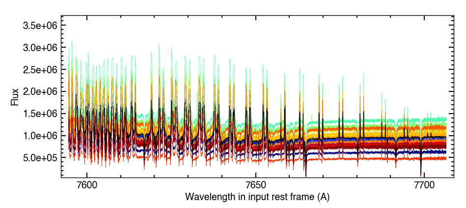
Fig. 15 Flux spectrum from one of the 2023-11-06 exposure, in ESPRESSO slices 164 and 165 typically affected by deep, poorly-corrected telluric lines (resulting in emission-like features from overcorrection). Most of the order was masked and excluded from further reduction. This plot was generated with plot_dic[‘flux_sp’] and is stored in …#
After setting up the masking you need to process the data again, by setting all modules up to this step to calculation mode (ie, gen_dic[‘calc_proc_data’], gen_dic[‘calc_gcal’], gen_dic[‘calc_corr_tell’]). We illustrate the masking in Fig. 14, where telluric CCFs are computed with the full spectral range (top) and masked spectral ranges (bottom).
Flux balance corrections#
This module resets the low-frequency profile of all spectra from the processed visits to the correct color balance. A global correction is performed over the full spectral range, and a second-order correction may then be applied within each order. We note that the overall flux level in each exposure will not be modified within this module.
Both corrections require defining a reference spectrum in each visit. Activate the Stellar masters submodule (gen_dic[‘glob_mast’]=True) and set it to calculation mode (gen_dic[‘calc_glob_mast’]=True).
The reference can be set to the mean or median of spectra measured over a selection of exposures (index idx_exp) in each visit:
gen_dic['glob_mast_mode']='mean' or 'med'
gen_dic['glob_mast_exp'] = {instrument:{visit: [idx_exp] }}
By default the master is computed as the median of all exposures in a visit. Alternatively you can use external spectra (e.g. if you know the true stellar spectrum), which must be defined for all visits using (see the configuration file for details):
gen_dic['glob_mast_exp'] = {instrument:{visit: file_path }}
Once the visit masters are defined, you can set the module to retrieval mode (gen_dic[‘calc_glob_mast’]=False).
Activate the Global flux balance submodule (gen_dic[‘corr_Fbal’]=True) and set it to calculation mode (gen_dic[‘calc_corr_Fbal’]=True).
This submodule fits the ratio between the full spectrum of each exposure and its corresponding visit master with a model, which is then used to set the spectrum to the master balance. When several visits are processed, as in the present example, a second correction is then applied toward the mean of the measured visit masters (default setting) or toward the external visit masters:
gen_dic['Fbal_vis']='meas' or 'ext'
Note
The first option is only possible when a single instrument is processed, and sets the spectra from all visits to a common color balance. The second option must be used when several instruments are processed because the measured master of a given instrument may not cover the full spectral range of another one.
The submodule can first be ran with its default settings. An iterative approach is then recommended to find the best fits for the flux balance models, which you can visualize by activating plot_dic[‘Fbal_corr’]=’pdf’ (for the intra-visit balance) and plot_dic[‘Fbal_corr_vis’]=’pdf’ (for the inter-visit balance). Look at the configuration file for details about each of the following settings, which you need to adjust through this iterative approach:
You can control the spectral bin size ‘Fbal_bin_nu’ of the fitted ratios, although the default value should be good enough in most cases.
A sigma-clipping is applied by default (gen_dic[‘Fbal_clip’]=True) to remove outliers. It is advised to perform a manual selection the spectral ranges (gen_dic[‘Fbal_range_fit’]) and/or spectral orders (gen_dic[‘Fbal_ord_fit’]) to exclude from the fit, such as:
gen_dic['Fbal_ord_fit'] = {'ESPRESSO':{'20231106': list(np.concatenate((range(2,88),range(92,145), range(148, 164),range(166,170)))),
                                       '20221117': list(np.concatenate((range(2,88),range(92,145), range(148, 164),range(166,170))))}}
Noisy ranges or orders (eg due to poor telluric correction from the previous module) will appear as outliers from the smooth flux balance ratios. If you use this setting, make sure that enough bins remain defined (especially at the bluest and reddest edges of the spectra) to constrain properly the flux balance model over the full spectral range to be corrected.
Phantom bins can be mirrored over a fixed range on each side of the measured spectra (here, gen_dic[‘Fbal_phantom_range’] = 10., in unit of \(c/\lambda\)) to limit the divergence of the fit.
Variance on fitted bins can be scaled to a power of gen_dic[‘Fbal_expvar’] (from 1 for original errors to 0 for equal weights). Bins in the blue part of the spectrum typically have large uncertainties and are not well captured by the fit. This scaling (here the default 0.25) increases the weight of the blue part of the spectrum with respect to the red part.
In parallel, choose the flux balance model best suited to your dataset and your goals. If flux balance variations are only at low frequency, if you suspect variations at medium frequency are not of Earth origin and worth investigating later one, or if you want to perform a first-order correction, you can use polynomial models and adjust the degree of the intra-visit and inter-visits (if relevant) corrections:
gen_dic['Fbal_mod']='pol'
gen_dic['Fbal_deg']={instrument:{visit:deg}}
gen_dic['Fbal_deg_vis']={instrument:{visit:deg}}
Otherwise you can use 1D smoothing splines and adjust the smoothing factor of the corrections:
gen_dic['Fbal_mod']='spline'
gen_dic['Fbal_smooth']={'ESPRESSO':{'20221117':1e-5,'20231106':1.1e-5}}
gen_dic['Fbal_smooth_vis']={'ESPRESSO':{'20221117':1.5e-4,'20231106':1.5e-4}}
This is the option that was preferred for the TOI-421 dataset given the medium-frequency variations that can be seen within each visit, and between both visits, in Fig. 16 (plots can be found in /Working_dir/Star/Planet_Plots/Spec_raw/FluxBalance/).
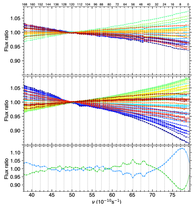
Fig. 16 Flux balance variations in TOI-421 spectra for the 2022-11-17 (top panel) and 2023-11-06 (middle panel) visits. Disks show the binned exposure spectra relative to the median reference in each visit. Exposures are colour-coded over the rainbow scale with increasing time, from purple to red. Matching colored lines show the fitted splines, which allow capturing subtle features, such as the ones visible around spectral order 112. The use of phantom bins avoids divergences in the blue part of the spectrum. The bottom panel shows the ratio between the median reference in each visit and their mean over both visits. These plots are automatically saved in: /Working_dir/Star/Planet_Plots/Spec_raw/FluxBalance/.#
Finally, you can choose the spectral ranges to be corrected for (with l in \(\\A\)):
gen_dic['Fbal_range_corr'] = [[l0,l1],[l1,l2],...]
Here we kept the default setting (gen_dic[‘Fbal_range_corr’]=[]) so that the entire spectra are corrected.
Once you are satisfied with the correction, set the submodule to retrieval mode (gen_dic[‘calc_corr_Fbal’]=False).
The next Order flux balance submodule performs a similar correction over each spectral order independently, to correct for local variations in Earth absorption or in the instrumental response.
It is controlled in the same way as the previous submodule, but is limited to fitting polynomial corrections (look at the configuration file for more information).
This correction must be used with caution, as it may also capture small-scale features of instrumental, stellar, or planetary origin.
Typically, it is not used with ESPRESSO spectra because it would capture part of their wiggle interference pattern, which are corrected for in a later module).
Cosmics correction#
Activate the Cosmics correction module (gen_dic[‘corr_cosm’]=True) and set it to calculation mode (gen_dic[‘calc_cosm’]=True).
The first step consists in choosing how to align (temporarily) the spectra so that they can be compared:
gen_dic['al_cosm']={'mode':'kep'}
The ‘kep’ option (default) uses the Keplerian model defined by the system properties you set up. The ‘pip’ option uses the RVs produced by the instrument DRS, if available. The ‘autom’ option cross-correlates the spectra, and requires defining the spectral ranges over which they are compared (‘range’ : [[l0,l1],[l2,l3],..], wich should cover enough deep and narrow stellar lines) and the RV range and step size used for cross-correlation (‘RVrange_cc’ : [min,max,step], which should cover the maximum range of RV shifts). The latter two options account for possible deviations from the Keplerian model, but will introduce biases in cases of strong Rossiter-McLaughlin anomalies.
Cosmic ray hits are identified by comparing the spectrum of interest with spectra taken in adjacent exposures, benefitting from the processing of consecutive time-series:
gen_dic['cosm_ncomp']=10
Here 5 exposures before (resp. after) the processed one will be used. Pixels are flagged as cosmics if their flux deviates from the mean of adjacent spectra by more than the pixel flux error, and the standard deviation over adjacent spectra, times a threshold, set as:
gen_dic['cosm_thresh'] = {'ESPRESSO':{'20221117':10,'20231106':10}}
This limits the risk of correcting pixels whose flux deviates due to the exposure noise alone. Cosmic-flagged pixels flux and error are then replaced by the mean and standard-deviation over adjacent spectra, respectively.
Tip
If your dataset displays large RV variations due, e.g., to a strong RM effect, use a small number of adjacent exposures to avoid blurring the flux of the corrected pixels.
You can select the indexes of exposures and orders to correct (by default left empty for full correction) with:
gen_dic['cosm_exp_corr']={instrument:{visit: [idx_exp] }}
gen_dic['cosm_ord_corr']={instrument:{visit: [idx_ord] }}
You can further choose to correct the n pixels on each side of the flagged ones (by default left empty for n = 0), to account for bleeding, with:
gen_dic['cosm_n_wings']={instrument:{visit: n }}
To inspect the quality of the cosmics correction you can plot the flux spectra (plot_dic[‘sp_raw’]=’pdf’) from each exposure, comparing the telluric-corrected (plot_settings[key_plot][‘plot_pre’]=’tell’) and cosmics-corrected (plot_settings[key_plot][‘plot_post’]=’cosm’) spectra.
You can further inspect the plots activated with plot_dic[‘cosm_corr’]=’pdf’ (saved in /Working_dir/Star/Planet_Plots/Spec_raw/Cosmics/Instrument_Visit/). Spectral detection profiles (ie, the ratio between the flux difference and error mentioned above) plotted for each exposure and order with cosmic-flagged pixels allow you to adjust the detection threshold (top panel in Fig. 17). The Occurrences plot (bottom panel in Fig. 17), which shows the number of flagged cosmic in each order over all exposures, is a good way to check if you are overcorrecting your dataset (typically if more pixels are flagged as cosmics toward the blue of the spectrum, where the noise is larger, or in lower S/R exposures).
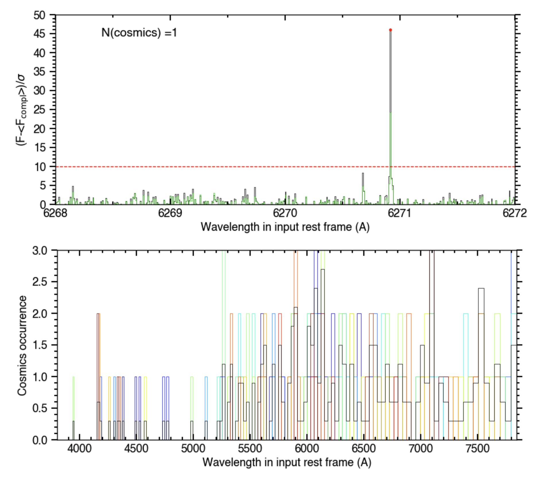
Fig. 17 Spectral detection profile (top panel) in the spectral order of an exposure in which a large deviation relative to 5 exposures before and after the exposure was flagged as a cosmic hit. Cosmic occurences per spectral order and exposure (colored over the rainbow scale, from purple to red) are shown in the bottom panel.#
Once you are satisfied with the correction, set the module to retrieval mode (gen_dic[‘calc_cosm’]=False).
Persistent peak masking#
This module is used to mask groups of pixels that show flux spikes persisting over time, typically hot detector pixels or sky emission lines that were not masked by the instrument DRS or removed by the sky-subtracted data.
The module relies on an estimate of the stellar continuum, calculated internally but using the settings of the Stellar continuum module.
Look into the stellar master tutorial how to adjust these settings.
Activate the Persistent peak masking module (gen_dic[‘mask_permpeak’]=True) and set it to calculation mode (gen_dic[‘calc_permpeak’]=True).
First, you need to define the exclusion settings. The module identifies pixels whose flux deviate from the stellar continuum by more than their error times a threshold:
gen_dic['permpeak_outthresh']=4
Then the module marks for masking a range centered on each flagged pixel, with width (in \(\\A\)) set as:
gen_dic['permpeak_peakwin']={instrument:width}
Finally a pixel is masked if it is marked in at least 3 consecutive exposures, or a larger number set as:
gen_dic['permpeak_nbad']=5
You can select the indexes of exposures and orders to be searched for peaks (by default left empty for full search) with:
gen_dic['permpeak_exp_corr']={instrument:{visit: [idx_exp] }}
gen_dic['permpeak_ord_corr']={instrument:{visit: [idx_ord] }}
You can further specify the spectral ranges (in \(\\A\)) to be searched within a given order with:
gen_dic['permpeak_range_corr'] = {instrument:{order: [[l1,l2],[l3,l4], ..] }}
Because the stellar continuum may not be well-defined toward the edges of spectral orders, you can also define a range to be excluded from the search on each side of the orders:
gen_dic['permpeak_edges'] = {instrument:[dl_blue,dl_red] }
Persistent peaks are rarely found in ESPRESSO data, and the module did not need to be used with the TOI-421 dataset. This correction may become relevant when processing near-infrared data, and the following plot were made from a transit dataset of XX observed with XX.
To inspect the quality of the peaks correction you can plot the flux spectra (plot_dic[‘sp_raw’]=’pdf’) from each exposure, comparing the cosmics-corrected (plot_settings[key_plot][‘plot_pre’]=’permpeak’) and peak-corrected (plot_settings[key_plot][‘plot_post’]=’cosm’) spectra.
You can also check the stellar continuum estimated within the module with plot_dic[‘permpeak_corr’]=’pdf’ (saved in …).
Once you are satisfied with the correction, set the module to retrieval mode (gen_dic[‘calc_permpeak’]=False).
Wiggle correction#
This module deals with the correction of interference patterns in ESPRESSO spectra, known as wiggles. Given the complexity of these patterns and their correction, we provide a dedicated tutorial.
Trimming#
This module is the last one of the reduction steps, and allows you to trim the spectra to a chosen range for the rest of the workflow. If your analysis only requires a specific spectral range, there is indeed no need to use computing time and storage space to process the full specra.
Activate the Trimming module (gen_dic[‘trim_spec’]=True) and set it to calculation mode (gen_dic[‘calc_trim_spec’]=True).
You can define which spectral ranges should be kept (with l in \(\\A\) in the solar barycentric rest frame) through:
gen_dic['trim_range'] = [[l1,l2],[l3,l4],..]
And/or which spectral orders should be kept through:
gen_dic['trim_orders'] = {instrument:{visit: [idx_ord] }}
The 2D echelle spectra now have comparable low-frequency profiles and are cleaned for environmental and instrumental effects.
You can set the present module to retrieval mode (gen_dic[‘calc_trim_spec’] = False) if you want to further process the spectral time-series. Otherwise the data can be retrieved for external use in the /Working_dir/Star/Planet_Saved_data/Corr_data/Trim/ directory.