
Getting started#
This page presents an overview of ANTARESS.
Spectroscopic time-series of standard spectrographs provided as input to ANTARESS can be retrieved as described here.
To help you familiarize with the workflow or run preliminary analyses you can run ANTARESS with dedicated notebooks.
To run semi-automatic analyses with minimal input on your part you can call ANTARESS with specific sequences.
Step-by-step tutorials detail how to process and analyze datasets for various purposes, using ANTARESS full capabilities.
Flowchart#
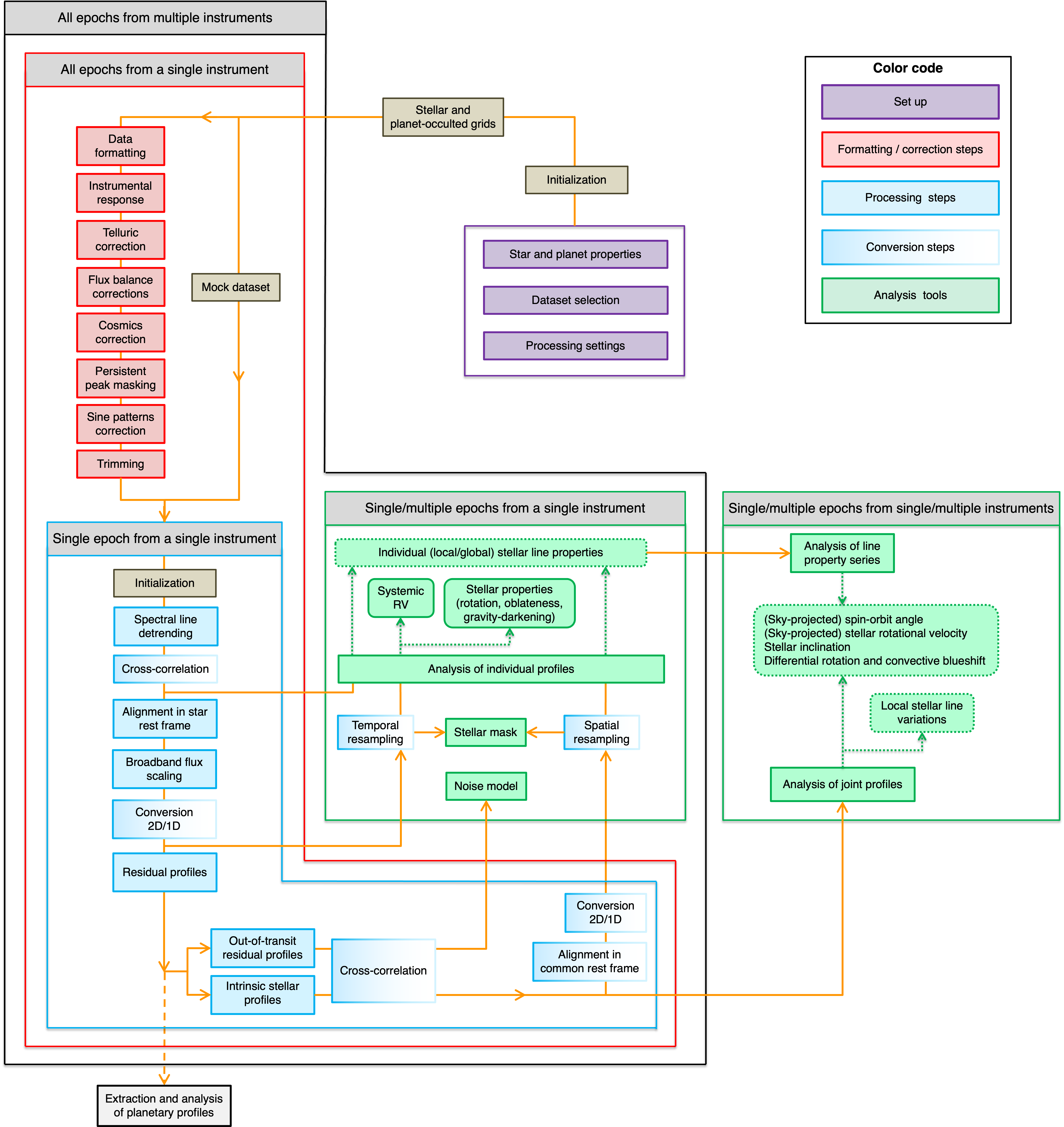
Fig. 1 Chart of the ANTARESS process flow.#
General approach#
Follow these steps to run ANTARESS:
Create a working directory and copy the following configuration files inside:
ANTARESS_systems.py: to define the system properties for the host star and its planets.
ANTARESS_settings.py: to configure the modules to process and analyze your input datasets.
ANTARESS_plot_settings.py: to define the settings controlling the plots from the workflow.
Move to the working directory and run the workflow from terminal with the command:
antaress --sequence sequence --custom_systems ANTARESS_systems.py --custom_settings ANTARESS_settings.py --custom_plot_settings ANTARESS_plot_settings.py
Alternatively you can run the workflow from your python environment as:
from antaress.ANTARESS_launch.ANTARESS_launcher import ANTARESS_launcher
ANTARESS_launcher(sequence = 'sequence' , custom_systems = 'ANTARESS_systems.py' , custom_settings = 'ANTARESS_settings.py' , custom_plot_settings = 'ANTARESS_plot_settings.py')
You can also run the workflow from any location by setting the option working_path to the path of your working directory.
The default configuration file contains pre-defined values that allow you to run the workflow with minimal intervention for a specific sequence. Any detailed analysis however requires that you customize those settings, following the step-by-step tutorials and leaving the sequence field undefined.
Processed data and fit results will be saved in a sub-directory /Star/Planet_Saved_data of the working directory, where Star and Planet are the name of the host star and planet(s) you defined in ANTARESS_systems.py.
Plots will be saved in a sub-directory /Star/Planet_Plots.
Copies of the default and custom configuration files will be saved in a sub-directory /Star/Settings_archive, with a specific timestamp for each run of the workflow.
Modules#
The workflow is organized as modules, which are grouped in three main categories (Fig. 1):
Formatting/correction: Data first go through these modules, some of which are specific to given instruments. Once data are set in the commonANTARESSformat and corrected for instrumental/environmental effects, they can be processed in the same way by the subsequent modules.Processing: The second group of modules are thus generic and aim at extracting specific types of spectral profiles, converting them in the format required for the analysis chosen by the user.Analysis: The third group of modules allow fitting the processed spectral profiles to derive quantities of interest.
Formatting/correction and Processing modules are ran successively, ie that data need to pass through an earlier module before it can be used by the next one. Analysis modules, in contrast, are applied to the outputs of various Processing modules throughout the pipeline.
Each module can be activated independently through the configuration file ANTARESS_settings.py. Some of the Formatting/correction and Processing modules are optional, for example the Telluric correction module for space-borne data or the Flux scaling module for data with absolute photometry.
Some modules are only activated if the pipeline is used for a specific goal, for example the CCF conversion of stellar spectra when the user requires the analysis of the Rossiter-McLaughlin effect.
In most modules you can choose to compute data (calculation mode, in which case data is saved automatically on disk) or to retrieve it (retrieval mode, in which case the pipeline checks that data already exists on disk).
This approach was mainly motivated by the fact that keeping all data in memory is not possible when processing S2D spectra, so that ANTARESS works by retrieving the relevant data from the disk in each module.
ANTARESS data outputs#
The data files output by ANTARESS are designed to be exploited internally within the workflow. They can however be easily retrieved from each module storage directory (given throughout the tutorials) within /Star/Planet_Saved_data.
All ANTARESS data files share a common structure, and can be opened as:
from antaress.ANTARESS_general.utils import dataload_npz
data = dataload_npz(file_path)
Most data files contain spectral profiles, which are stored as matrices with the following fields:
data[‘cen_bins’] : center of spectral bins (in \(\\A\) or km/s) with dimension [ \(n_{orders}\) x \(n_{bins}\) ]
data[‘edge_bins’] : edges of spectral bins (in \(\\A\) or km/s) with dimension [ \(n_{orders}\) x \(n_{bins}+1\)]
data[‘flux’] : flux values with dimension [ \(n_{orders}\) x \(n_{bins}\) ]
data[‘cond_def’] : definition flags (True if flux is defined) with dimension [ \(n_{orders}\) x \(n_{bins}\) ]
data[‘cov’]: banded covariance matrix with dimension [ \(n_{orders}\) x [ \(n_{diag}\) x \(n_{bins}\) ] ]. For more details, see Bourrier et al. 2024, A&A, 691, A113 and the bindensity package.
Where orders represent the original spectrograph orders for data in echelle format, or a single artificial order for 1D spectra and CCFs.
Plots#
Plots are generated at the end of the workflow processing, upon request.
At the end of each module in the main configuration file ANTARESS_settings.py you can activate a given plot_name by setting plot_dic[‘plot_name’] to an extension, such as pdf.
Some plots require specific outputs, which are not produced by default due to their large size. This means that if you activate a plot after running the workflow once and retrieving its results, it may not compute. You will simply have to run the workflow again in calculation mode for the relevant modules.
The plot settings are then controlled through the plot configuration file ANTARESS_plot_settings.py. All plots have default settings, but a large number of options are available so that you can adjust the plot contents and their format.