
Wiggle correction#
This tutorial is part of the spectral reduction steps.
This module offers two methods to correct for the ESPRESSO wiggles, using either an analytical model over a full visit dataset (preferred approach), or a filter in each exposure. The analytical model describes a beat pattern between two sine-like components, which are dominating the wiggle pattern in most ESPRESSO datasets. Because this model only describes the wiggle signal and is constrained by all exposures, it prevents overfitting and provides a robust and homogeneous correction between ESPRESSO datasets. The filter approach is more efficient and easier to set-up, but introduces the risk of overcorrecting planetary and stellar features at medium spectral resolution. It should be limited to observations in which the wiggle pattern is too complex to be captured with the analytical model.
Activate the ESPRESSO "wiggles" module (gen_dic[‘corr_wig’]= True) and set it to calculation mode (gen_dic[‘calc_wig’] = True).
Initialization#
Wiggles are processed as a function of light frequency (\(\nu = c/\lambda\)), to be distinguished from the frequency F of the wiggle patterns. Here we go through the initialisation settings that are common for both the analytical and filter method.
Wiggle corrections are applied on a visit-by-visit basis since there is currently no clear correlation of the wiggle pattern between visits. Specify which visits to process within:
gen_dic['wig_vis'] = ['20221117','20231106']
Wiggles are characterized on transmission spectra, calculated as the ratio between each exposure spectrum and a stellar master spectrum. You usually want to correct for wiggles in all exposures, but may choose to exclude some of them from the building of the master. You can manually specify the indexes of the master exposures using (leave empty to use all exposures):
gen_dic['wig_exp_mast'] = {'20231106' : [exp0, exp1, ...]}
All spectra in this module are resampled to compute transmission spectra at lower spectral resolution, to smooth out high-frequency noise and reduce computing time. The default bin size (in \(10^{13}\) Hz) is suited to the main wiggle components:
gen_dic['wig_bin'] = 0.0166
If you suspect or want to search for additional wiggle components at higher frequency, you may decrease the bin size.
Screening#
This first step is common to both the analytical and filter correction approaches. It serves two purposes:
Identifying the exposures and spectral ranges to be included in the analysis (i.e., where wiggles are significant compared to noise)
Determining which wiggle components affect your dataset.
Activate the screening submodule with gen_dic[‘wig_exp_init’]= {‘mode’: True}. For initial tests, you can leave the other submodule settings at their default values. They control two diagnostic plots (generated by default):
The spectral ratios between each exposure spectrum and a chosen master (i.e., transmission spectra). An additional setting allow you to control the vertical range of the plots, otherwise determined automatically.
A periodogram of the wiggle power, considering all exposures together, to identify the number and approximate frequency of the wiggle components
Plots of are automatically saved in the /Working_dir/Star/Planet_Plots/Spec_raw/Wiggles/Instrument_Visit/Screening/ directory.

Fig. 3 Transmission spectrum in one of the 20221117 exposures, as a function of light frequency. The wiggle pattern is clearly visible, but dominated by noise at the center and blue end of the spectrum. The spectrum is colour coded by spectral order.#
Based on the plotted transmission spectra, determine the exposures to include in the wiggle characterization (‘all’ will select all of them):
gen_dic['wig_exp_in_fit'] = {
           '20221117': 'all',
           '20231106': list(np.delete(range(54),[5])),
       }
Excluding an exposure, as in the above arbitrary example, may be relevant if it is too noisy to contribute to the wiggle characterization, or if it displays an outlying wiggle pattern. Since the wiggle pattern evolves slowly over the typical duration of a few exposures, you also have the possibility to characterize the model over groups of exposures defined as:
gen_dic['wig_exp_groups'] = {
            visit : [ [exp0, exp1] , [exp2 , exp3 , exp4] , .. ] }
       }
While it is not useful in the case of the TOI-421 datasets, it can be relevant useful when individual transmission spectra are too noisy to characterize the wiggle pattern properly, especially toward the bluest orders. Finally, perform an initial identification of the spectral ranges to be included in the fit and select them with:
gen_dic['wig_range_fit'] = {
           '20221117': [[20.,57.1],[57.8,67.3] ],
           '20231106': [[20.,50.6],[51.1,54.2],[54.8,57.1],[57.8,67.3] ],
       }
You need to exclude ranges exhibiting high noise levels relative to the wiggle amplitude). As illustrated in Fig. 3, wiggles usually decrease in amplitude toward the blue of the spectrum, where the S/N also decreases (as the flux gets lower due to Earth diffusion and the black body of typical exoplanet host stars). You thus need to decide beyond which light frequency the transmission spectra do not bring any more constraints to the wiggle characterization and may degrade the overall fit quality. Here we chose \(\nu\) = 6.73 x \(10^{13}\) Hz. Wiggles are also typically dominated by noise toward the center of the center of the spectrum (\(\nu \sim\) 57-58 x \(10^{13}\) Hz) at the edges of the blue and red detectors.
Tip
Although this is not the case in this example, some datasets may display an additional wiggle pattern with lower frequency and localized S-shaped features (typically at \(\nu \sim\) 47, 51, 55 x \(10^{13}\) Hz). The current version of the analytical model does not account for this pattern. You can either ignore them, if they fall in a range you do not plan on analyzing, or follow the approach described in the next section.
The final transmission spectrum with the excluded regions should show some clear periodic signals, as shown in Fig. 4.
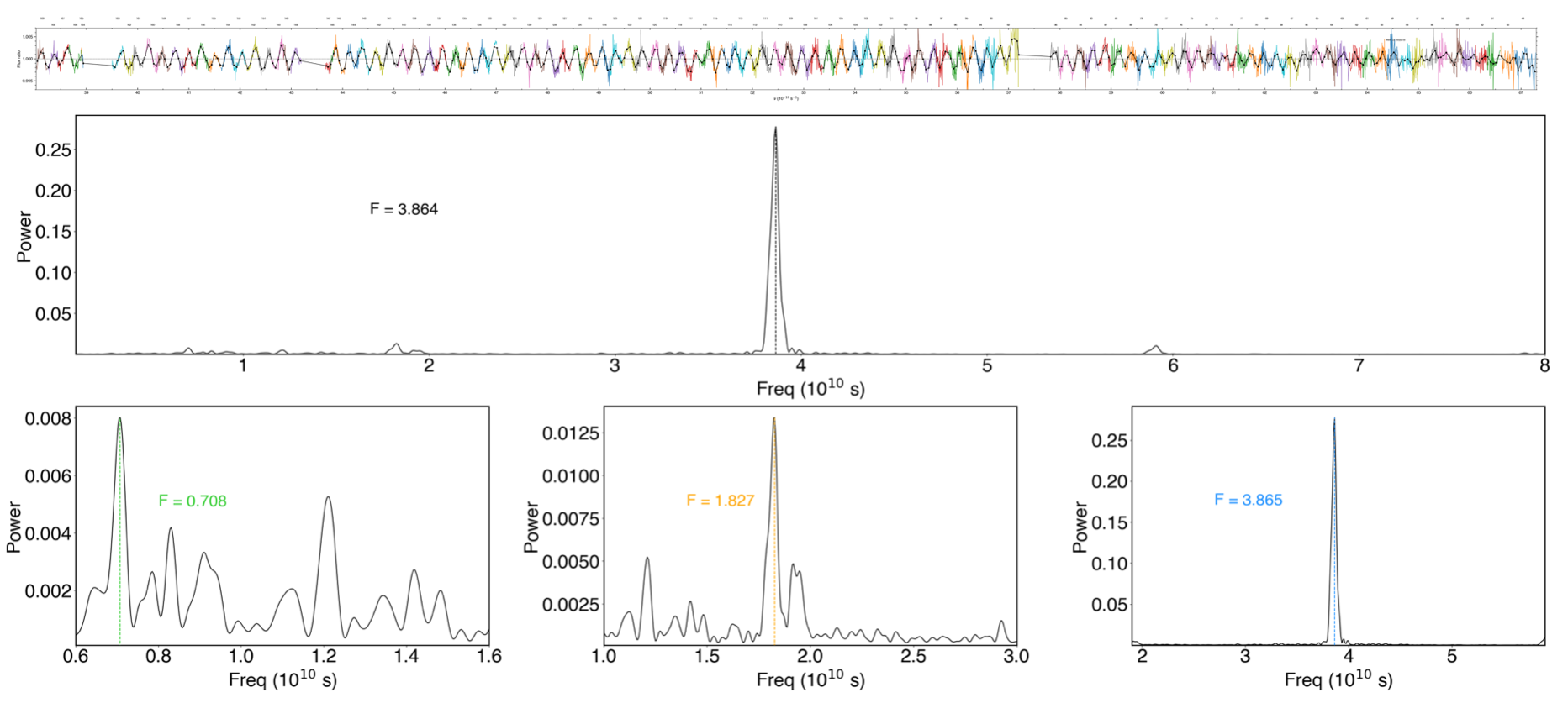
Fig. 4 Final transmission spectrum after removing regions with significant noise. The bottom panel shows the mean periodogram computed for all exposures from the observation.#
After excluding spectral ranges with high noise levels, the wiggle pattern and associated peaks in the periodogram should become clearly visible, as shown in Fig. 4. If they remain indistinct, wiggles may be small enough that a correction is not required. Otherwise you can now deactivate this step (gen_dic[‘wig_exp_init’]= {‘mode’: False}) and move on to either the filter or analytical correction.
Method 1: filter#
Activate the filter approach by setting mode to True in:
gen_dic['wig_exp_filt']={
        'mode':True,
        'win':0.3,
        'deg':4,
        'plot':True
        }
Define values for the filter smoothing window (‘win’) and polynomial degree (‘deg’) that are fine enough to capture the wiggle pattern without overfitting spurious features in the data.
The plot field allows you to adjust the filter settings by inspecting the transmission spectum and its associated periodogram (saved in the /Working_dir/Star/Planet_Plots/Spec_raw/Wiggles/Instrument_Visit/Filter/ directory), as shown in Fig. 5.

Fig. 5 Transmission spectrum before and after filtering.#
A drawback of this approach is that it may smooth out spectral features and potentially remove signals of planetary or stellar origin. However, this method allows you to isolate and correct specific spectral ranges in which unexpected features may appear that cannot be modeled analytically. After this correction, you can then re-inject into the wiggle module the corrected spectra and apply the analytical model.
Method 2: Analytical model#
Analysis of multiple datasets have shown that wiggles are best described as the sum of multiple sinusoidal components. The wiggle pattern can be expressed as:
\(W(\nu, t) = 1 + \sum _k A_k(\nu, t) \sin(2\pi \int (F_k(\nu,t)d\nu ) - \Phi_k(t)).\)
And is usually dominated by two main components. This module follows an iterative approach to determine the best-fitting parameters to model these components. The first two key properties to estimate are the frequencies and amplitudes of each component, denoted as \(F_k(\nu)\) and \(A_k(\nu)\), respectively. They are expressed as polynomial expansions:
\(A_k (\nu, t) = \sum_{i=0}^{d_{a,k}} a_{\text{chrom},k,i}(t)(\nu - \nu_{\text{ref}})^i\),
\(F_k (\nu, t) = \sum_{i=0}^{d_{f,k}} f_{\text{chrom},k,i}(t)(\nu - \nu_{\text{ref}})^i\).
Where:
\(A_k(\nu,t)\) represents the amplitude variation as a function of light frequency and time.
\(F_k(\nu,t)\) represents the frequency variation as a function of light frequency and time.
\(\nu_\text{ref}\) is a light frequency reference used for normalization.
\(d_\text{a,k}\) and \(d_\text{f,k}\) define the polynomial order for amplitude and light frequency variations.
The coefficients \(a_\text{chrom,k,i}(t)\) and \(f_\text{chrom,k,i}(t)\) capture the chromatic dependence of the amplitude and light frequency, respectively.
\(\Phi_k(t)\) represents the phase offset of the sinusoidal component at time \(t\).
When using the analytical model, you may better capture the wiggle pattern by enforcing normalization of the transmision spectra in each spectral order with gen_dic[‘wig_ana_norm_ord’] = True.
Two important events may occur during an observing night, which will impact the wiggle pattern and its characterization with the analytical model:
Meridian crossing : we found out that when the line-of-sight toward the star crosses the meridian, the temporal variation of the wiggle model parameters remains continuous but changes in derivative.
Guide star change : ESPRESSO observations with the VLT rely on a guide star. We found out that when it is changed during an observing sequence, the wiggle pattern changes entirely. This translates into a reset of all wiggle model parameters, introducing a discontinuity in their temporal variation at the time of the change. While this effect is accounted for in
ANTARESS, we strongly recommend to ask ESO support astronomers to use the same guide star within an observing sequence.Tip
If the wiggle model parameters appear to remain continuous over time despite a guide star change, you can deactivate its automatic identification by including the visit in the gen_dic[‘wig_no_guidchange’] list. This can also be useful in cases where only a small number of exposures are available on one side of the guide star change, making it difficult to independently characterize the wiggle parameters, and in cases when the guide star change occurs near the meridian crossing, where allowing both a derivative and parameter reset in close succession can introduce too much flexibility into the model. You can assess whether this setting is appropriate by examining the result of Step 4.
Step 1: Sampling Chromatic Variations#
In the screening step you identified spectral regions that can be used to constrain the wiggle pattern and assess the strength of its components. In this step, activated with gen_dic[‘wig_exp_samp’][‘mode’]= True, you will sample the chromatic variations of the wiggle component across a representative set of exposures. This means sampling the frequency and amplitude of each component as a function of light frequency \(\nu\).
First, select a set of exposures to sample using:
gen_dic['wig_exp_in_fit'] =  {
   '20221117':np.arange(0,28,5),
   '20231106':np.arange(0,54,5)}
Tip
Since the wiggle pattern evolves relatively slowly with time, we do not need to sample their variations in every exposure. For the TOI-421 datasets, we thus sample one every fifth exposure.
In narrow bands, the wiggles can be approximated by a sine with constant frequency and amplitude. The sampling is thus performed automatically by sliding a fixed window over a given transmission spectrum, and at each sampled position:
Apply a periodogram to estimate the local wiggle frequency \(F_k(\nu)\).
Fit a sine function at this frequency to estimate the local wiggle amplitude \(A_k(\nu)\).
The window size must be large enough to include several oscillation cycles of the wiggle pattern. Furthermore, we recommend overlapping successive windows to sample more finely the wiggle pattern.
This is an iterative process. Once the first component is processed, the piecewise model built over the sliding windows is used to temporarily correct the transmission spectrum (Fig. 6). The second component can then be sampled and analysed in the same way (Fig. 7). We describe below the settings controlling this process, using the 20221117 visit as example.
Process the highest-frequency component by setting:
gen_dic['wig_exp_samp']['comp_ids'] = [1]
Once this first component is analysed, you will correct it and process the second component by setting [1,2]. You need to provide an estimate of each component frequency \(F_k(\nu)\), described as a polynomial with coefficients ci:
gen_dic['wig_exp_samp']['freq_guess']:{
        1:{ 'c0':3.72, 'c1':0., 'c2':0.},
        2:{ 'c0':2.05, 'c1':0., 'c2':0.}}
Approximating \(F_k(\nu)\) to a constant is usually sufficient for this step, and the above values should be similar for other datasets. This guess frequency is also used to calculate the width of the sliding window, which is set by the number of cycles you want to sample for each component:
gen_dic['wig_exp_samp']['nsamp'] = { 1 : 8 , 2 : 8 }
The oversampling of the sliding windows is controlled by shifts in \(\nu\) (in \(10^{13} s^{-1}\)) set as:
gen_dic['wig_exp_samp']['sampbands_shifts'] = {
    1:np.arange(16)*0.15,
    2:np.arange(16)*0.30 }
The pipeline loops over the shifts, positions the first window at the lowest \(\nu\) of the spectrum plus the shift, and then slides the window over consecutive (non overlapping) positions. When processing the second component, the first one is corrected for using the piecewise model built over the sliding windows positioned for a given shift, whose index within sampbands_shifts is set as:
gen_dic['wig_exp_samp'][2] = 0
Periodograms associated with each window are searched for the peak wiggle frequency over a broad default range (‘mod’:None), or within a range (in \(10^{13} s^{-1}\)) centered on the guess \(F_k(\nu)\) for this window:
gen_dic['wig_exp_samp']['src_perio']={
        1:{'mod':'slide','range':[0.5,0.5] ,'up_bd':False },
        2:{'mod':'slide','range':[0.5,0.5] ,'up_bd':True  }}
Where ‘up_bd’:True restricts the range upper boundary for the second component to the first component frequency. The sine fit is then only performed in the window if the FAP of its peak periodogram frequency is below a threshold (in %):
gen_dic['wig_exp_samp']['fap_thresh'] = 5
To better converge on the sine fit it is repeated iteratively gen_dic[‘wig_exp_samp’][‘nit’] times.
You can improve the quality of the sampling after having completed Step 3, by fixing the frequency of the components (here the first) to its value from the best-fit model in each exposure:
gen_dic['wig_exp_samp']['fix_freq2expmod'] = [1]
And after having completed Step 5, by fixing the frequency of the components to their values from the best-fit model in each visit (stored at a given path):
gen_dic['wig_exp_samp']['fix_freq2vismod'] = {
    comps:[1,2] ,
    '20221117' : 'path1/Outputs_final.npz',
    '20231106' : 'path2/Outputs_final.npz' }
The gen_dic[‘wig_exp_samp’][‘plot’] field plots the sampled transmission spectra and sampling analyses, stored under /Working_dir/Star/Planet_Plots/Spec_raw/Wiggles/Exp_fit/Instrument_Visit/Sampling/.
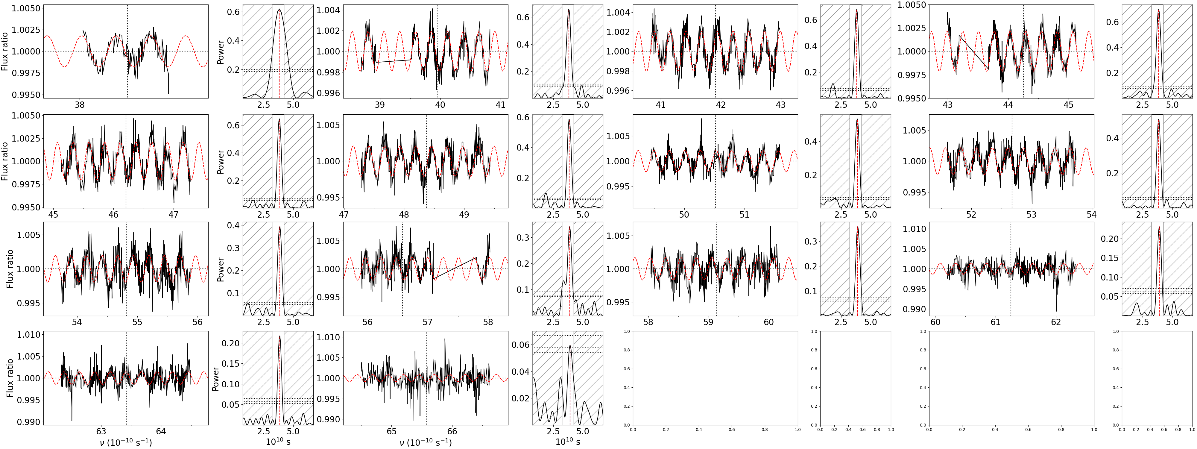
Fig. 6 Sampling of the first wiggle component in the 20221117 visit.#
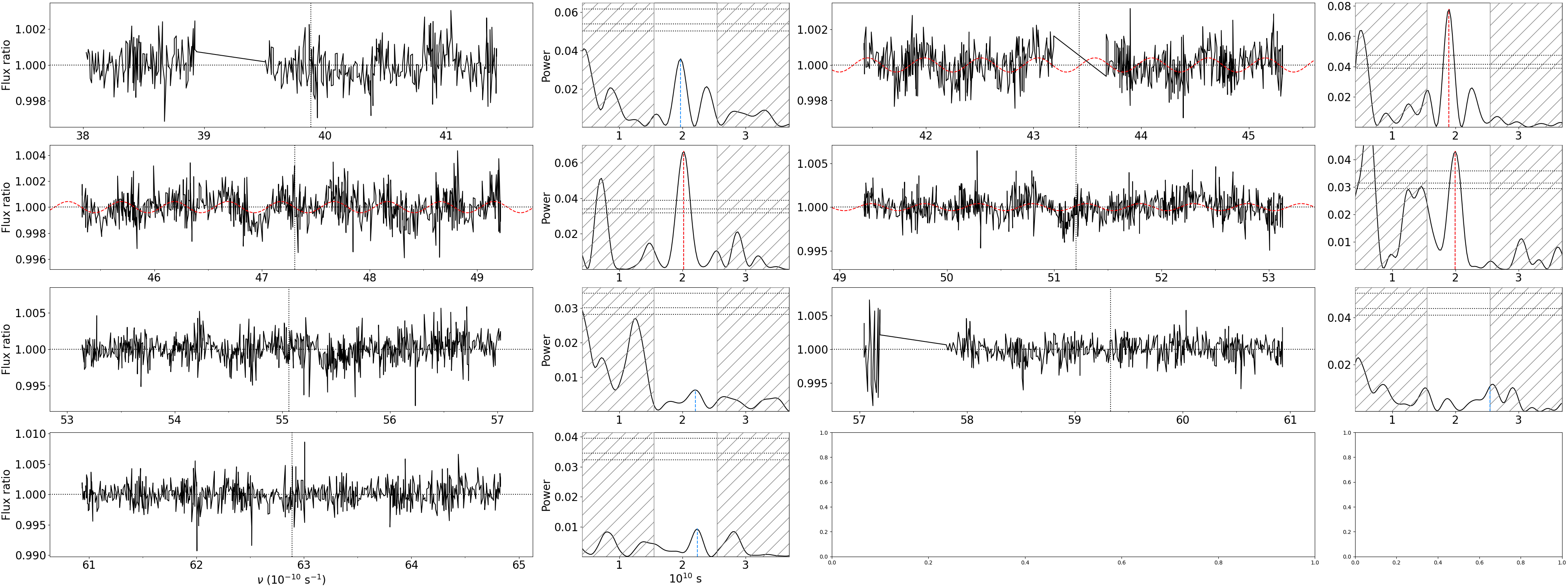
Fig. 7 Sampling of the second wiggle component in the 20221117 visit. The piecewise model built from the sampling of the first component has been corrected for.#
You can now deactivate this step (gen_dic[‘wig_exp_samp’][‘mode’]= False) and move on to the next one.
Step 2: Chromatic analysis#
In the previous step we sampled the variations of the wiggle frequency \(F_k(\nu)\) and amplitude \(A_k(\nu)\) with \(\nu\) in a selection of exposures. We now analyze those variations to determine the appropriate degrees for the polynomials describing \(F_k(\nu)\) and \(A_k(\nu)\).
Activate the submodule by setting ‘mode’ to True in
gen_dic['wig_exp_nu_ana']={
    'mode':True,
    'comp_ids':[1,2],
    }
The ‘comp_ids’ field allows you to select the wiggle components to characterize, among those you detected in the previous steps. The polynomial degrees are set with:
gen_dic['wig_deg_Freq'][1] = 1
gen_dic['wig_deg_Freq'][2] = 0
gen_dic['wig_deg_Amp'][1] = 2
gen_dic['wig_deg_Amp'][2] = 2
In most cases the wiggle frequency and amplitude are well described using linear and quadratic functions, respectively. The second (low-frequency) component typically has lower amplitudes and may be characterized with lower precision than the first (high-frequency) component, requiring only a constant frequency (as in the case of the TOI-421 dataset).
Tip
In reality the wiggle pattern likely requires higher polynomial degrees to be described over the full ESPRESSO range. In high-quality datasets the pattern may be characterized with Step 1 and Step 2 even at shorter wavelengths (higher \(\nu\)). In most datasets this is not possible, but you can try and evaluate in Step 3 whether higher degrees provide a better fit to the full transmission spectra.
To find the appropriate polynomial degree, test different values and manually inspect the diagnostic plot (Fig. 8) activated by setting gen_dic[‘wig_exp_nu_ana’] to True. These plots are automatically saved in /Working_dir/Star/Planet/Spec_raw/Wiggles/Exp_fit/Instrument_Visit/Chrom/.
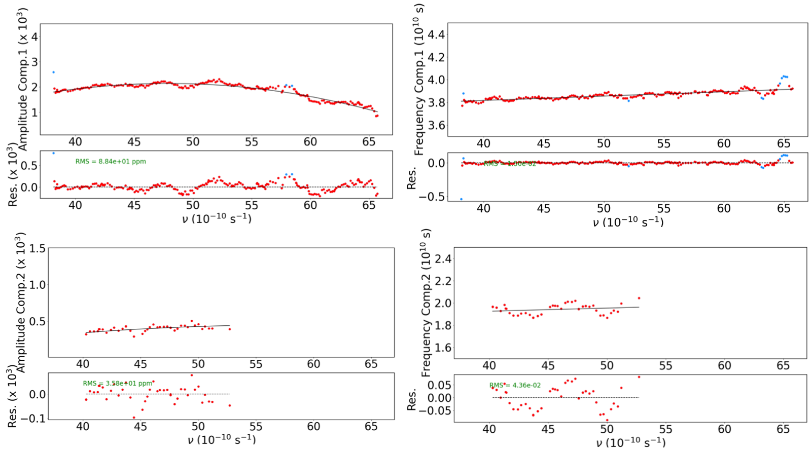
Fig. 8 Chromatic analysis of the amplitude and frequency for the first and second wiggle components in the TOI-421 dataset. Amplitude is best described as a second-degree polynomial for the first component (top left panel), and as a linear function for the second component (bottom left panel). Frequency is best described linearlyt for both components (right panels).#
To improve the fit you can automatically exclude outliers by setting a threshold for sigma-clipping as:
gen_dic['wig_exp_nu_ana']['thresh'] = 3.
Excluded outliers are flagged in blue in the plots, for visual confirmation.
At this stage, it is useful to review the initial screening and fitting steps before proceeding. By examining the diagnostic plots you can spot regions that are poorly fitted, typically showing sharp deviations in the sampled values over narrow \(\nu\) intervals. This may indicate that you need to adjust the sliding window used in Step 1, or that you exclude additional spectral regions from the analysis in the Screening.
You can now deactivate this step (gen_dic[‘wig_exp_nu_ana’][‘mode’]= False), and move on to the next one.
Step 3: Exposure fit#
In this step we fit the spectral wiggle model \(W(\nu,t)\) to each exposure independently, to estimate time-series for the phase shift \(\Phi(t)\) and chromatic coefficients \(a_{\text{chrom},k,i}(t)\) and \(f_{\text{chrom},k,i}(t)\) (which describe the wiggle frequency \(F_k(\nu)\) and amplitude \(A_k(\nu)\)).
Activate the submodule by setting ‘mode’ to True in
gen_dic['wig_exp_fit']={
   'mode':True,
   'comp_ids':[1,2],
   'init_chrom':True,
    }
The ‘comp_ids’ field allows you to select the wiggle components to include in the model, which can be useful to assess whether using an additional wiggle component actually improves the fit.
The ‘init_chrom’ field initializes the fitted chromatic coefficients to the rough estimates derived in the previous step, improving the convergence of the fit and the accuracy of the results. If you activate this field make sure that Step 2 is applied to the same ‘comp_ids’ components as defined here.
Tip
The module initializes the coefficients fitted in a given exposure to those derived for the closest exposure in time among those analyzed in Step 2. This is why you only need to run the previous step over a representative selection of exposures sampling the temporal variations of the coefficients.
If you skip the previous step or do not want to use the ‘init_chrom’ option, you can manually provide guess estimates for the frequency chromatic coefficients as:
gen_dic['wig_exp_fit']={
   'freq_guess':{
       1:{ 'c0':3.72, 'c1':0., 'c2':0.},
       2:{ 'c0':2.05, 'c1':0., 'c2':0.}},
    }
For example, you can provide a constant frequency based on the periodogram from the Screening step (as above), or all polynomial coefficients based on the analysis in the next steps.
Some options in this step rely on the model derived in the subsequent step. For the first run, these options should be left empty. It is best to use an iterative approach between this and the next step (Step 4).
Further keywords for the setting concerns the fitting procedure with: nit, number of iterations, fit_method either ‘leastsq’ or ‘nelder’ if convergence is difficult to reach, use to calculate or retrieve fits.
You can use priors on fitted parameters by indicating the parameter and boundaries as:
gen_dic['wig_exp_fit']['prior_par']['vis'] = {'par0': [min, max],
                                              'par1': [min, max]}
By using the next submodule Pointing analysis you can further constrain the model by using the values derived as priors or as fixed values. With the model from the next step Pointing analysis you can either keep values fixed to their model value using:
gen_dic['wig_exp_fit']['fixed_pointpar']['vis'] = [prop0, prop1,...]
Or you can use the model derived and base your priors around it as:
gen_dic['wig_exp_fit']['model_par']['vis'] = {par : [-val, +val]}
Which is interpreted as the interval around the model for each parameter defined here. To asses the model and correction plots are automatically saved in /Working_dir/Star/Planet/Spec_raw/Wiggles/Exp_fit/Instrument_Visit/Global/.
Combining the submodules Exposure fit and Pointing analysis we used the following settings and priors for TOI-421 night 20221117.
gen_dic['wig_exp_fit']={

   'init_chrom':True,
   'freq_guess':{
       1:{ 'c0':3.8, 'c1':0., 'c2':0.},
       2:{ 'c0':2.0, 'c1':0., 'c2':0.}
       },
   'nit':20,
   'fit_method':'leastsq',
   'use':True,
   'fixed_pointpar':{},
   'prior_par':{},
   'model_par':{},
   'plot':True,
   }

gen_dic['wig_exp_fit']['model_par']['20221117']={
           'AmpGlob1_c0':[0.3e-4,0.3e-4],
           'AmpGlob1_c1':[0.3e-5,0.3e-5],
              'Freq1_c0':[0.0004,0.0004],
              'Freq1_c1':[0.00025,0.00025],
              'Freq2_c0':[0.02,0.02],
                  'Phi1':[0.1,0.1],
                  'Phi2':[0.5,0.5],
       }
By applying the model and analyzing the resulting corrections, you can assess the model’s performance before moving on to the next step. If you still notice prominent spikes in the periodogram after applying the correction, it’s a good idea to examine the areas where the model fails. In some datasets, using a higher-degree polynomial in the chromatic analysis may be necessary to achieve a better fit in the higher-frequency range and improve the correction of the wiggle pattern.

Fig. 9 Exposure fit example for the visit on 20221117: The periodogram at the top shows a strong peak, which disappears in the residuals after the correction.#
The resulting plots are automatically saved in: /Working_dir/Star/Planet/Spec_raw/Wiggles/Exp_fit/Instrument_Visit/Global/. You can now deactivate this step (gen_dic[‘wig_exp_fit’][‘mode’]= False), and move on to the next one.
May need to come back to previous step: + + Continue to the next step, Exposure Fit, to assess how well the model performs across different spectral regions, particularly where the chromatic analysis showed significant variations.
Step 4: Pointing Analysis#
In this step, each parameter fitted during the Exposure Fit is evaluated as a time series and modeled against the telescope’s pointing coordinates. This allows us to characterize the pointing-dependent terms in the final model, including the chromatic coefficients \(a_{\text{point},k,i}(t)\) and \(f_{\text{point},k,i}(t)\), as well as the phase shift \(\Phi_{\text{point},k,i}\). The model derived here can also be used directly as priors using the ‘model_par’ option, or use the model to find appropriate priors, additionally you can fix values for parameters for an additional run of the Exposure Fit, making it useful to iterate between these two steps to refine the parameters and achieve model convergence. To calculate the model for the pointing of the telescope activate the submodule gen_dic[‘wig_exp_point_ana’][‘mode’] = True.
The evolution of the first component for amplitude, frequency, and phase shift can be seen in Fig. 10, for TOI-421 night 20221117. A key feature of this model is the discontinuity that occurs at the time of a guide star change. This event is explicitly accounted for in the model, as all parameters are reset at the moment of the guide star switch. Because this discontinuity can significantly affect the wiggle modeling, it is best examined at this stage.
However, in some datasets the discontinuity may be negligible or occur near the beginning or end of the observation window. In such cases, it may be appropriate to deactivate the parameter reset by including the night in the ‘wig_no_guidechange’ field at the start of the wiggle module.
For the fitting procedure, you can select the source of the fitting coefficients—either from the Exposure Fit results by setting ‘glob’, or from the sampling results using ‘samp’. At this stage, it may also be beneficial to include more exposures in the fit by removing the initial grouping applied at the beginning of the module. This can be done using the ‘wig_exp_in_fit’ field. However, note that changing the set of exposures in this way requires re-running Step 3: Exposure Fit, which will increase computational time. Despite the added cost, fitting the model using the full set of exposures may be necessary to achieve optimal results.
Additional tools to improve the pointing model include:
Automated outlier removal, which can be enabled by setting a threshold with ‘thresh’
Skipping undefined parameters using ‘fit_undef’
Specifying a custom range for fitting particular parameters or visits, using:
gen_dic[‘wig_exp_point_ana’][‘fit_range’] = {vis : {par :[low, high]}}
For parameters that show poor convergence or no clear trend with the pointing coordinates, you can fit them as constants by listing them in the ‘stable_pointpar’ field. This is especially useful for stabilizing the model when certain components do not exhibit meaningful time or pointing dependence.
Keep in mind that the amplitude and phase values are degenerate and periodic with \(\pi\), which can lead to apparent discontinuities in the phase plots. These discontinuities often arise when the final model value includes a phase shift that is an integer multiple of \(\pi\). When this happens, the corresponding amplitude values will also show a sign flip if the phase shift involves an odd multiple of \(\pi\), which inverts the sign of the amplitude for that data point in the model. To automatically correct for this effect, you can activate the option ‘conv_amp_phase’, which adjusts the amplitude sign based on the detected phase discontinuities.
Tip
The pointing analysis is based on the parameters derived in the previous step, Exposure Fit. Once you have a model for the pointing analysis, you can further refine the model by using it as the basis for your priors in the exposure fit. Model priors are calculated from the model \(v(t)\) as \([v(t) - \text{model_par}[0], v(t) + \text{model_par}[1]]\). By analyzing the model (see :numref:pointing_analysis) for each component, you can adjust the constraints for the priors until you achieve a good model and fit.
Here is how priors and the model priors were set up for the analysis of night 20221117:
 gen_dic['wig_exp_fit']['prior_par']['20221117']={
        'AmpGlob2_c0':{'low':-4e-3,'high':4e-3},
        'AmpGlob2_c2':{'low':-1e-7,'high':1e-7},
           'Freq1_c0':{'low':3.84,'high':3.8575},
           'Freq2_c0':{'low':1.7,'high':2.2},
               'Phi2':{'low':-30.,'high':30.},
    }
gen_dic['wig_exp_fit']['model_par']['20221117']={
        'AmpGlob1_c0':[0.3e-4,0.3e-4],
        'AmpGlob1_c1':[0.3e-5,0.3e-5],
           'Freq1_c0':[0.0004,0.0004],
           'Freq1_c1':[0.00025,0.00025],
           'Freq2_c0':[0.02,0.02],
               'Phi1':[0.1,0.1],
               'Phi2':[0.5,0.5],
    }
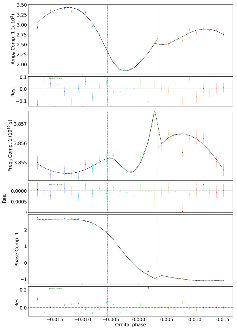
Fig. 10 Pointing analysis displaying the time evolution of the main component of the three functions \(a_{\text{point},k,i}(t)\), \(f_{\text{point},k,i}(t)\), and \(\Phi_{\text{point},k,i}\). The gray vertical dashed line indicates the pointing passing the meridian and the vertical black dashed line represents a change of guide star. You can further see how the model changes behaviour around these two points, where the change of guide star introduces a discontinuity in the model.#
The resulting plots are automatically saved in: /Working_dir/Star/Planet_Plots/Spec_raw/Wiggles/Exp_fit/Instrument_Visit/Coord/.
The model derived in this step can be used to create model priors with a uniform distribution around the model value for each exposure when recomputing the exposure fit.
- The vertical lines in the pointing analysis represent critical time steps in the pointing and wiggle model.
When passing the meridian, the derivatives of the model parameters reset completely.
The change of guide star results in a complete reset of model parameters unless the option gen_dic[‘wig_no_guidchange’] is used to ignore this reset.
You can now deactivate this step (gen_dic[‘wig_exp_point_ana’][‘mode’]= False), and move on to the next one.
Step 5: Global visit fit#
The full spectro-temporal wiggle model \(W(\nu, t)\) is initialized using the results from the previous step and fitted to all exposures simultaneously. Due to the large number of free parameters and the complexity of a model composed of cumulative sine functions, it is crucial to provide guess values close to the best-fit solution to ensure proper convergence.
gen_dic['wig_vis_fit']={
    'mode':False ,
    'fit_method':'leastsq',
    'wig_fit_ratio': False,
    'wig_conv_rel_thresh':1e-5,
    'nit':15,
    'comp_ids':[1,2],
    'fixed':False,
    'reuse':{},
    'fixed_pointpar':[],
    'fixed_par':[],
    'fixed_amp' : [],
    'fixed_freq' : [],
    'stable_pointpar':[],
    'n_save_it':1,
    'plot_mod':True    ,
    'plot_par_chrom':True  ,
    'plot_chrompar_point':True  ,
    'plot_pointpar_conv':True    ,
    'plot_hist':True,
    'plot_rms':True ,
    }

# Fields below are only relevant if nested sampling is used for parameter estimation ('fit_method' = 'ns')
gen_dic['wig_vis_fit']['ns'] = {
    'nthreads': int(0.8*cpu_count()), ### number of threads for nested sampling
    'run_mode': 'use',
    'nlive': {}, # If empty (nlive = 50 * N_free)
    'resume':''
}
Note
Parameter descriptions:
- fit_method specifies the optimization method to use for fitting:
‘leastsq’: Fast and sufficient if the initialization is correct.
‘nelder’: More robust but slower, useful when convergence is difficult.
‘ns’: Uses nested sampling (currently under development).
nit number of fit iterations to perform. A higher value allows for better convergence but increases computation time.
comp_ids nefines which model components to include in the fit. This allows selecting specific terms of the model to optimize.
- fixed determines whether the model parameters are kept fixed during fitting:
True: The model remains fixed to the initialization or previous fit results.
False: The parameters are free to vary during fitting.
- reuse specifies whether to reuse a previous fit file:
{}: No reuse.
Path to a fit file: The file is retrieved for post-processing (fixed=True) or used as an initial guess (fixed=False).
fixed_pointpar list of pointing parameters that should remain fixed during the global fit.
fixed_par list of general model parameters that should remain fixed during the fit.
fixed_amp specifies a list of components whose amplitudes should remain fixed during fitting.
fixed_freq specifies a list of components whose frequencies should remain fixed during fitting.
stable_pointpar list of pointing parameters that should be fitted with a constant value instead of varying across exposures.
n_save_it frequency at which fit results are saved (every n_save_it iterations). Helps track progress and recover data in case of interruptions.
plot_hist generates a cumulative periodogram over all exposures to visualize residual periodic structures before and after correction.
plot_rms plots the RMS (root mean square) of pre/post-corrected data over the entire visit to assess the effectiveness of the correction.
Applying the correction#
In this step, the spectro-temporal wiggle model correction is applied to the data. This correction uses the model derived from the global fit and applies it across the relevant spectral range(s) and exposures.
This step must be applied regardless of whether you are using the filter method or the analytical method for the final correction.
gen_dic['wig_corr'] = {
    'mode':False,
    'path':{},
    'exp_list':{},
    'comp_ids':[1,2],
    'range':{},
    }
Note
Parameter descriptions:
mode enables or disables the correction step. Set to True to apply the correction.
path specifies the path to the correction file for each visit. If left empty ({}), the most recent result from ‘wig_vis_fit’ is used. Result files from
Global fitare stored in: /working_dir/Star/Planet/Corr_data/Wiggles/Vis_fit/Instrument_Visit/. Format used is: ‘path’:{‘visit’:’file_path’}.exp_list defines which exposures to correct for each visit. If left empty ({}), the correction is applied to all exposures.
comp_ids list of components to include in the correction. These components must be present in the global fit model (wig_vis_fit).
range specifies the spectral range(s) (in Å) over which the correction should be applied. If left empty ({}), the correction is applied to the full spectrum.
To visually assess the correction, use the plotting dictionary plot_dic[‘trans_sp’] to check the transmission spectra. Ensure that the wiggle patterns have been properly removed. In the plot_settings file, under ‘trans_sp’, set [‘plot_pre’]=’cosm’ to plot the spectrum before the correction (after cosmic correction), and [‘plot_post’]=’wig’ to plot the spectrum after the wiggle correction.